Degree Distribution of Arbitrary AANET
Abstract
Taking the safe distance between two adjacent planes in the same airline into account, we give a model for the multiairline aeronautical ad hoc network (AANET). Based on our model, we analyze the plane’s degree distribution of any arbitrary AANET. Then, the expressions of the degree distributions of one single plane and the whole networks are both worked out and verified by the simulations, in which we generate several random AANETs. Since our model is a reasonable abstraction of the real situation, the theoretical result we get is very close to the result of the real networks, which is also shown in the simulations.
1. Introduction
With the rapid development of civil aviation, the demands of accessing Internet on board have become stronger than ever before. However, in polar, desert, marine, and other areas where base stations cannot be built, aircrafts have to use satellite links or large span multihop links within AANET to reach base stations. Due to the large delay, high cost, and limited bandwidth of satellite links, AANET is preferred for internet accessing in these regions [1, 2].
For AANET, the Newsky project has proposed networking strategies with mobile IPv6 technology [3]. ATENAA project (advanced technologies for networking in aeronautical applications) has studied Ka-band array antennas and optical communications between aircrafts [4]. Rohrer et al. have presented cross-layer networking solutions among physical, mac, network, and transport layers [5]. Vey et al. have proposed the use of direct sequence CDMA (DS-CDMA) at the access layer [2] while Yan et al. have studied the capacity of single flight path AANET [6].
In an ad hoc network, the number of a node’s neighbors is called “degree” of that node. Thus, the degree distribution of an ad hoc network tells the probability that the degree is an exact number by choosing a node randomly. Based on the degree distribution of the network, a lot of work can be done: the analysis of connectivity and robustness of the network by using the method of generating function formalism [7]; the design of routing and mac protocols; for example, we can choose planes with high degree expectation to relay messages, since usually we cannot know where all the planes are; the site selection of base stations; for example, base station can be set at a place to make sure that the average of the degree expectations of planes in coverage region of that base station is high, which makes it reach more planes through multihop links.
The degree distribution of mobile ad hoc networks has been widely discussed, but most of them are based on the scenarios that nodes in the networks move randomly. However, for AANET and vehicle ad hoc networks (VANET), the nodes are moving along specified lines, which is different from the old scenarios. In VANET, which is also studied a lot in recent years, the speed of vehicles can be affected by plenty of factors (such as pedestrian crosswalks, traffic jams, and traffic lights) and the degree distribution which a vehicle is hard to calculate or even to assume. Thus, the problem about calculating the degree distribution of the networks where nodes move along specified lines has not been solved yet.
In this work, we give a model for the AANET, from which we can approximately calculate the degree distribution of any arbitrary AANET.
2. The Model
Since AANET is not deployed currently and none of the achievements mentioned previously is taken as standard or in real use, we do not consider the physical or access layer of AANET and use a fixed value, r (between 50 nmi and 300 nmi as used in [8]), as the communication range for all planes.
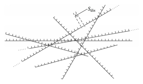
According to the specifications of the International Civil Aviation Organization (ICAO) [9], a safe distance, call it Sdis (it is around 20 nmi according to ICAO), should be kept between two adjacent planes in the same airline. As the length of an airline is far greater than Sdis, we take Sdis as the smallest unit of length. Thus, we assume that the distance between two adjacent planes in the same airline can only be kSdis (k = 1,2, 3, …). Since the distance of two airlines at different height level is usually several hundred of meters, which is much less than the assumed planes’ communication range r, we ignore the distance of two airlines.
In Figure 1, there are several random lines crossing each other with points uniformly spaced on them. The lines stand for airlines while points denote the possible locations of planes. The distance between two adjacent points in the same line is Sdis. Furthermore, we assume that the spatial distribution of planes on each airline obeys discrete uniform distribution.
3. The Degree Distribution of a Plane
The usual method to calculate the degree distribution of a plane is experimentally based on the scenario that the spatial distribution of planes in each airline follows Poisson point process, and it is easy to tell that the degree distribution of a plane obeys Poisson distribution [6, 10]. However, the scenario does not take the nonignorable safe distance between planes into account, which is significantly different from the real situation in the sky. For instance, in [6, 10], the number of a plane’s neighbors can be infinite, but if safe distance is considered, the number of each plane’s neighbors has an upper limit.
In Figure 2, there are m airline segments covered by plane F (m equals 3 in this example). In each segment, there are several possible locations for planes and we denote ni as the number of locations in segment i (i = 1,2, …, m), where the location occupied by plane F is not counted. For each location of segment i, we denote Pi as the probability that a plane is at that location.
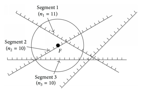
Since planes can only be at the designed locations on the airlines, the probability that plane F has K neighbors is the probability that K planes are at the locations covered by plane F. Then, using ki (ki ∈ [0, ni]) to denote the number of planes on segment i, we can get and the probability that there are ki planes on segment i is , where denotes the number of the ways of setting ki planes at ni locations.
In order to set K planes in total at the locations covered by plane F, we set planes following this order: k1 to segment 1, k2 to segment 2, and km to segment m. Thus, the value ranges of k1 to km are as shown in Table 1.
| ki | Value range |
|---|---|
| k1 | [0, min(n1, K)] |
| k2 | [0, min(n2, K − k1)] |
| k3 | [0, min(n3, K − k1 − k2)] |
| ⋮ | ⋮ |
| kh |
|
| ⋮ | ⋮ |
| km |
|
4. The Degree Distribution of AANET
5. Numeric Results
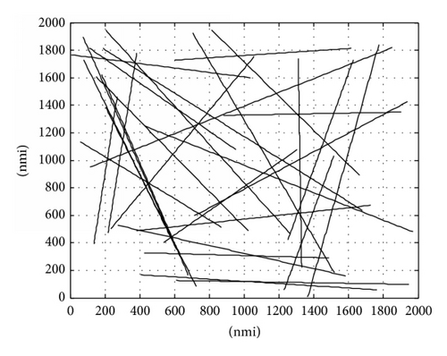
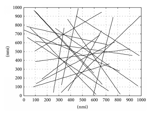
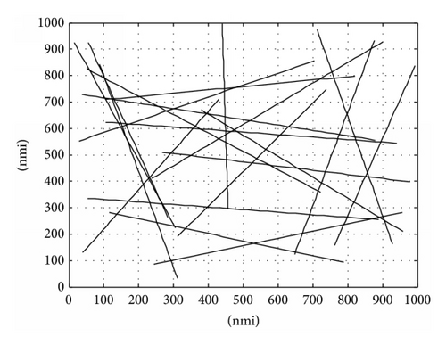
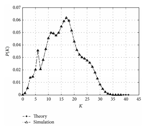
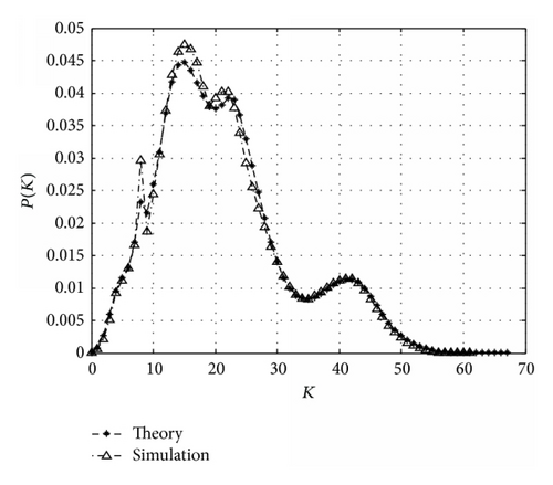
We calculate the theoretical value in (5) and simulation value in (6) for each scenario in Figures 3 to 5 and draw their results in Figures 6 to 8, respectively, where the theory and simulation lines are overlapped.
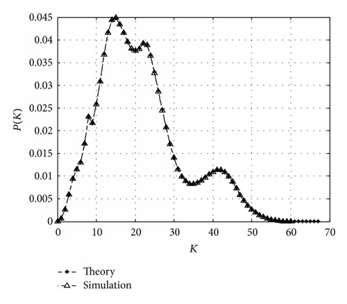
From Figures 6 to 8, we can see that the probability that a plane has no neighbor is nearly zero, because a plane at most of the locations (except the locations near the endpoints of the airlines) can cover at least 6 locations in its own airline in scenarios 2 and 3 (r = 70 nmi, Sdis = 20 nmi) and 10 locations in scenario 1 (r = 100 nmi, Sdis = 20 nmi). With considering that every Pi we choose is larger than 0.5, the probability that a plane has no neighbor should certainly be very small. Another thing we can tell from the figures is that the probability decays to zero for large degrees. As we inform in Section 3, the number of each plane’s neighbors has an upper limit since a safe distance should be kept between two planes. When a plane’s degree reaches the upper limit, this means that every location covered by that plane should have a plane on it. Thus, when the upper limit is big, the probability of reaching that limit should be very small and, for the degrees beyond the maximum upper limit, it should be zero.
The peaks of Figures 7 to 9 are related mostly on the communication range and safe distance, because those two parameters decide how many locations a plane can cover; for example, plane at most of the locations (more than 50%) in scenario 1 can cover over 15 to 20 locations (counted by computer), so the peak of scenario 1 should most likely be around 15 and 20, and Figure 6 proves that, for scenarios 2 and 3, they are 10 to 20 and 15 to 22, respectively.
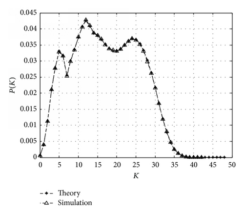
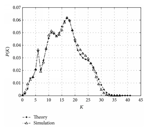
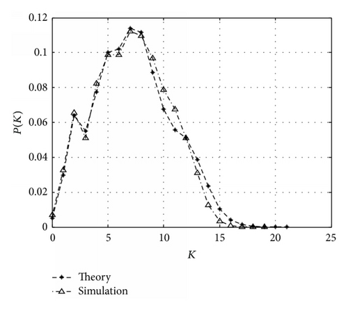
Since, in the real world, planes cannot be exactly at the locations we draw in our scenarios, we give a random shift for every plane after each generation of planes. Then, we run the simulation again to see the deviation between our theoretical model and the real situation. The results are shown in Figures 9 to 11 and the random shift strategy is described in the following paragraph.
For each airline, we move its first plane (left most plane) a distance of L1 along the airline, where L1 is uniformly distributed between −Sdis/2 and Sdis/2. For the second plane, we move it a distance of L2. L2 has two different distributions according to whether it is at the location adjacent to the first plane’s or not. If yes, L2 is uniformly distributed between L1 and Sdis/2 to make sure the distance of the two planes is not less than Sdis. If no, L2 has the same distribution of L1. Following this way, we move the jth plane according to whether the (j − 1)th and jth planes are at the adjacent locations on that airline.
From Figures 9 to 11, we can see there is only a small deviation between our model and the real situation, and it is believed to be decreasing with the ratio of r to Sdis. In Figures 10 and 11, we use the same scenario with different safe distances. The shapes of the two figures are similar, but the mathematical expectation of K in Figure 10 is nearly the double of that in Figure 11. This is because scenario can form the shape, while safe distance can decide the plane density.
6. Conclusion
In this paper, we introduce a model of AANET, which considers the nonignorable safe distance between planes. Based on this model, the plane’s degree distribution of an arbitrary AANET is analyzed. We find that, different from other works, the degree of each plane in our model has an upper limit, which is coursed by the safe distance. Then, we get from the numeric results of our theoretical method that the peaks of the degree distribution are related mostly on the communication range and safe distance, and the probability of getting large values of degree is very small and it is zero for the degrees beyond the maximum upper limit.
For future research, we will consider simulating a network around some real-world flight paths as opposed to changing the distribution of random paths to show the utility of our method in a real-world case.
Conflict of Interests
The authors declare that there is no conflict of interests regarding the publication of this paper.
Acknowledgments
This research is supported by the National Natural Science Foundation of China (Grants nos. 61171089, 91438104, and 61302054) and Chongqing Science & Technology Commission (Grants nos. cstc2014yykfA40002 and cstc2012jjb40010).
Appendix
| Airline | Range of x | P | |
|---|---|---|---|
| 1 | 2.58x + y − 1929.54 = 0 | [77.95,613.29] | 0.6 |
| 2 | 0.76x + y − 1178.04 = 0 | [58.39,879.89] | 0.89 |
| 3 | 0.02x + y − 139.37 = 0 | [608.17,1953.46] | 0.89 |
| 4 | 0.04x + y − 342.61 = 0 | [427.14,1489.82] | 0.82 |
| 5 | −4.49x + y + 6127.43 = 0 | [1364.92,1776.88] | 0.95 |
| 6 | 0.50x + y − 1461.92 = 0 | [429.48,1979.71] | 0.75 |
| 7 | −0.88x + y + 69.05 = 0 | [536.53,1311.26] | 0.72 |
| 8 | −1.52x + y − 146.88 = 0 | [233.33,1059.16] | 0.53 |
| 9 | −7.97x + y + 692.72 = 0 | [135.93,270.73] | 0.65 |
| 10 | 1.24x + y − 2958.86 = 0 | [811.29,1665.92] | 0.73 |
| 11 | −3.49x + y + 3939.50 = 0 | [1251.73,1628.00] | 0.55 |
| 12 | 0.16x + y − 1768.40 = 0 | [7.73,1035.99] | 0.74 |
| 13 | 0.79x + y − 1962.16 = 0 | [187.84,1679.15] | 0.69 |
| 14 | −3.42x + y + 4146.90 = 0 | [1229.30,1520.74] | 0.52 |
| 15 | −0.02x + y − 1306.39 = 0 | [880.62,1911.55] | 0.87 |
| 16 | 0.08x + y − 200.58 = 0 | [405.60,1777.07] | 0.64 |
| 17 | 2.50x + y − 1897.33 = 0 | [204.49,731.02] | 0.77 |
| 18 | 2.93x + y − 2154.74 = 0 | [180.99,683.54] | 0.75 |
| 19 | 0.88x + y − 1912.86 = 0 | [109.41,953.64] | 0.57 |
| 20 | 1.39x + y − 2231.38 = 0 | [203.71,1264.09] | 0.55 |
| 21 | 79.68x + y − 106171.04 = 0 | [1310.57,1329.72] | 0.51 |
| 22 | 1.28x + y − 1800.32 = 0 | [151.01,1028.81] | 0.77 |
| 23 | −7.95x + y + 1258.15 = 0 | [217.53,383.32] | 0.53 |
| 24 | 2.14x + y − 3430.21 = 0 | [703.89,1519.09] | 0.67 |
| 25 | 0.28x + y − 603.50 = 0 | [274.77,1588.72] | 0.74 |
| 26 | −0.09x + y − 1677.97 = 0 | [599.14,1635.26] | 0.55 |
| 27 | −0.14x + y − 435.09 = 0 | [379.64,1737.19] | 0.83 |
| 28 | −0.50x + y − 892.90 = 0 | [113.78,1862.92] | 0.87 |
| 29 | 2.88x + y − 2110.97 = 0 | [74.49,603.50] | 0.96 |
| 30 | −0.68x + y − 111.87 = 0 | [713.92,1950.68] | 0.95 |
| Airline | Range of x | P | |
|---|---|---|---|
| 1 | 1.35x + y − 844.70 = 0 | [55.61,620.46] | 0.53 |
| 2 | 0.30x + y − 792.12 = 0 | [25.45,725.70] | 0.66 |
| 3 | −0.40x + y − 66.80 = 0 | [80.66,747.52] | 0.73 |
| 4 | −5.24x + y + 3096.09 = 0 | [592.50,761.51] | 0.73 |
| 5 | 0.93x + y − 1012.40 = 0 | [269.63,980.69] | 0.81 |
| 6 | −6.06x + y + 1825.23 = 0 | [321.40,464.85] | 0.69 |
| 7 | 0.19x + y − 635.55 = 0 | [99.68,928.24] | 0.6 |
| 8 | −8.03x + y + 1991.97 = 0 | [252.56,346.31] | 0.53 |
| 9 | −1.29x + y + 375.77 = 0 | [319.11,998.05] | 0.82 |
| 10 | −1.01x + y − 31.62 = 0 | [155.09,650.33] | 0.91 |
| 11 | 1.90x + y − 1575.72 = 0 | [374.37,826.71] | 0.55 |
| 12 | −0.18x + y − 369.57 = 0 | [98.74,915.06] | 0.56 |
| 13 | 0.57x + y − 745.92 = 0 | [0.62,816.80] | 0.66 |
| 14 | −0.71x + y − 61.87 = 0 | [104.25,782.36] | 0.81 |
| 15 | −2.39x + y + 847.86 = 0 | [377.03,665.98] | 0.71 |
| 16 | 0.88x + y − 688.99 = 0 | [31.63,723.34] | 0.79 |
| 17 | −0.78x + y − 433.04 = 0 | [94.40,673.71] | 0.84 |
| 18 | 1.44x + y − 1092.75 = 0 | [86.99,676.56] | 0.83 |
| 19 | 0.83x + y − 1274.48 = 0 | [446.49,991.50] | 0.73 |
| 20 | 1.40x + y − 1092.81 = 0 | [97.50,597.67] | 0.91 |
| Airline | Range of x | P | |
|---|---|---|---|
| 1 | 2.89x + y − 1085.85 = 0 | [55.84,286.33] | 0.86 |
| 2 | 0.09x + y − 633.54 = 0 | [104.28,954.11] | 0.71 |
| 3 | −1.30x + y + 213.65 = 0 | [311.92,743.70] | 0.57 |
| 4 | 0.79x + y − 971.51 = 0 | [378.87,967.53] | 0.88 |
| 5 | −0.78x + y − 224.71 = 0 | [237.94,912.15] | 0.74 |
| 6 | −2.94x + y + 2079.82 = 0 | [761.69,998.72] | 0.98 |
| 7 | 0.16x + y − 552.34 = 0 | [268.09,986.72] | 0.94 |
| 8 | 0.20x + y − 736.46 = 0 | [37.21,896.98] | 0.58 |
| 9 | −0.13x + y − 696.10 = 0 | [105.55,824.21] | 0.91 |
| 10 | 2.41x + y − 961.32 = 0 | [14.72,311.12] | 0.83 |
| 11 | 0.10x + y − 340.86 = 0 | [53.07,905.06] | 0.94 |
| 12 | 3.63x + y − 1161.00 = 0 | [87.59,315.56] | 0.9 |
| 13 | −3.54x + y + 2166.35 = 0 | [647.85,880.35] | 0.75 |
| 14 | −0.45x + y − 539.45 = 0 | [28.99,709.69] | 0.83 |
| 15 | 0.28x + y − 313.95 = 0 | [114.26,795.89] | 0.77 |
| 16 | −0.28x + y − 17.43 = 0 | [243.10,971.41] | 0.87 |
| 17 | 3.75x + y − 3643.45 = 0 | [711.96,929.24] | 0.82 |
| 18 | −1.49x + y − 71.08 = 0 | [39.60,432.18] | 0.87 |
| 19 | 0.69x + y − 860.79 = 0 | [50.20,724.29] | 0.76 |
| 20 | 41.71x + y − 19333.33 = 0 | [439.63,456.41] | 0.55 |


