We construct dynamic Bertrand-Stackelberg pricing models including two manufacturers and a common retailer in a risk-averse supply chain with the uncertain demand. The risk-averse supply chain follows these strategies: Bertrand game between the two manufacturers and Stackelberg game between the manufacturer and the retailer. We study the effect of the price adjustment speed, the risk preference, and the uncertain demand on the stability of the risk-averse supply chain using bifurcation, power spectrum, attractor, and so forth. It is observed that there exists slip bifurcation when the price adjustment speed across some critical value, the stable region, and total profit of the risk-averse supply chain will increase with increase of and decrease with increase of σ. The profit of the supply chain and the two manufacturers will decrease and the weaker (retailer) is a beneficiary when the supply chain is in chaos. The fluctuation in the supply chain can be gradually controlled by the control of the price adjustment speed.

1. Introduction

With the development of economic globalization, the relationship among the supply chain members becomes more and more complex under the different environment. An enterprise which is involved in the middle of multiple supply chains has all kinds of complicated relationship when the parameter of the upstream and downstream enterprises is changed, such as market uncertainty and risk preference factor; the enterprise’s decision-making behaviors become more complicated and hard to predict.

We all know that the price is always a sensitive topic, which can affect customer needs and wants, distribution of the products and services among the supply chains. Scholars at home and abroad have done a lot of research on this aspect. Wei et al. [1] studied pricing decisions in a supply chain with two manufacturers and one common retailer and constructed five pricing models under decentralized decision cases with consideration of different market power structures. Mukhopadhyay et al. [2] considered two separate firms, which had private forecast information about market uncertainties and offered complement goods in a leader-follower type, and devised a “simple to implement” information sharing scheme under which both firms and the total system are better off. These literatures analyzed and compared the optimal solution under different market power structures, but they did not consider the effect of risk reference of the participants on the optimal solution.

There are many literatures taking risk preference into account. Caliskan-Demirag et al. [3] constructed models of the supply chain with a risk-averse retailer by adopting the conditional-value-at-risk (CVaR) decision criterion. Luo and Huang [4] explored the impact of risk preference on the strategies of the supply chain by taking the different attention of high profit and low profit as retailers risk measurement. These literatures only consider the unilateral risk, but, in the uncertainty environment, there exists bilateral risk among the participants which corresponds to the actual situation. In this paper, we will consider a supply chain under bilateral risk with two risk-averse manufacturers and a risk-averse retailer, which make the supply chain more complex.

Many literatures study the complexity of supply chain. Huang and Chen [5] studied the sale-surety contract option of supply chain with effort dependent demand and risk preference and got some meaningful conclusions. Guan and Zhou [6] researched the integrated optimization problem of three-level supply chain consisting of suppliers, distributors, and retailers under decision-makers having different risk attitude. Huang and Yang [7] studied a two-echelon supply chain model with one supplier and one retailer in a newsvendor problem; the supplier with different risk attitude has great influence on the retailer’s optimal order quantity; the operation efficiency of the supply chain will be underperformed when the supplier is much too risk-averse. These literatures have studied the participant’s behaviors of the risk supply chain, but they did not present the dynamic complex features of the risk supply chain.

Research on dynamical complexity of a system has been of concern to scholars. Puu [8] found that the Cournot three oligopoly model could appear strange attractors with fractal dimension, and he studied the situation of the duopoly game. Many researchers improved the classical Cournot model and found that certain dynamical behaviors of the system occurred in the course of repeated games with three or four duopolies. Many experts have also studied this field under different conditions, such as different expectations and incomplete information select it Ma and Sun [9] established a decentralized pricing game model and studied its complex dynamic characteristics of triopoly under different decision-making rule; the result showed that the process of game would tend to a Nash equilibrium at a lower price adjustment speed, and, with the increase of the value of adjustment speed, the system would appear to be unstable and gradually gone into a chaos state. Ma and Bangura [10] studied the dynamic complexity of financial and economic system under the condition of three parameters changing.

In recent years, many experts apply the dynamical complexity to study the dynamic change process of supply chain. Hwarng and Xie [11] found that there existed the chaotic enlargement phenomenon among the members of the supply chain which enriched the connotation of the bullwhip effect. J. Wang and X. Wang [12] established nonlinear supply chain inventory system models with forbidden returning and limited supply capacity; numerable simulations showed that the supply chain inventory system had complex dynamic behaviors under certain parameter settings; they gave some suggestions to eliminate the complexity of the dynamic supply chain. Ma and Feng [13] presented investigation simulations of retailer’s demand and stock; the behaviors of the system exhibited deterministic chaos with consideration of system constraints. These literatures researched the dynamic complexity of the supply chain but did not consider the influence of the decision-maker’s risk behaviors on the supply chain management. In this paper, we will study the dynamic complexity of a risk-averse supply chain with two manufacturers and a common retailer under uncertain demand. Considering the change of parameters in the dynamic risk supply chain, such as the price adjustment speed, risk preference, and uncertain demand, we can study the influence of parameters on the price and stable region of the two manufacturers and retailer.

The remainder of this paper is organized as follows. In Section 2, we describe the supply chain problem, make assumptions of the system model, and discuss the system model. In Section 3, we construct a Bertrand-Stackelberg dynamic pricing model which consists of two manufactures and one retailer with risk-averse attitude. Analysis is made under different variable conditions in Section 4. In Section 5, the variable feedback control method will be used to control chaos in the system. In Section 6, we outline some conclusions and hence relevant recommendations for future research.

2. Model

2.1. Description of the Problem

In this section, we construct a dynamic pricing game model in a risk-averse supply chain which consists of two manufacturers (M₁ and M₂) and a common retailer (R). The two manufacturers are competitive and sell respective products to the common retailer, and the common retailer sells two kinds of products to consumers directly. The customers’ demand is stochastic. We consider the supply chain following these strategies: Bertrand game between the two manufacturers and Stackelberg game between the manufacturer and the retailer. In these strategies, the two manufacturers and the retailer make their own decisions, respectively, for maximizing their profit; the decision process is as follows: the two manufacturers, as the Stackelberg leader, determine the respective wholesale price (w_i) (i = 1,2); the retailer as the follower sets his own optimal retail price (p_i) (i = 1,2) based on the manufacturer’s decisions.

Furthermore, in order to capture the uncertain demand which is affected by the change of economic and business conditions and prediction errors, we assume the market demand random variable a is as follows: , where is the primary demand level and ε follows a normal distribution such as E(ε) = 0, Var⁡(ε) = σ². However, the normality assumption has been used extensively in the literature (e.g., Gal-Or [14]; Raju and Roy [15]; Vives [16]). The two manufacturers and the retailer know the distribution of the uncertain demand and determine their behaviors, respectively.

Because the customer demand is stochastic, there is financial risk to the two manufacturers and the retailer. Therefore, we should consider the effect of the risk preference of the two manufacturers and the retailer on pricing decision. The preference theory provides the framework which incorporates the participators’ financial risk preference into their decision process. The valuation measure we use is known as the certainty equivalent in the preference theory and is defined as certain value that a participator is just willing to accept an uncertain event (Kunstman [17]).

One form of the utility function in both theoretical and applied work in areas of decision theory and finance is the exponential utility function which can be expressed as (i = M₁, M₂, R), where R_i is the risk tolerance level of the two manufacturers and retailer, π_i is the profit, and e is the exponential constant. When R_i < ∞, it implies that the decision-maker has risk-averse behavior, and R_i approaches ∞ which implies the decision-maker is risk-neutral (Walls [18]). If the decision-maker is risk-averse, π follows a normal distribution, and expected utility is E(U) = E(π) − (Var⁡(π)/2R), where E(π) is the mean of π and Var⁡(π) is the variance of π.

2.2. Assumption of the System

(1)
Customer demand is always satisfied, demand function is linear, and the two manufacturers and the retailer make decentralized decision.
(2)
We consider two partly substitutable products coming from a competitive market in which consumers can buy any one of them.
(3)
The consumer demand is stochastic; the two manufacturers and the retailer are all risk aversion.
(4)
is marginal cost of M₁; is marginal cost of M₂.

2.3. Revenue Function of the System

In this study, w_i and p_i (i = 1,2) are decision variables and other variables are exogenous variables. As is known in the supply chain, we assume that p_i ≥ w_i (i = 1,2); this inequality ensures that each participant can obtain a positive profit.

Extend the demand function in Banker et al. [19]. We assume that the primary demand function in this paper is decided by p_i (i = 1,2) as follows:

()

where a represent the base demand level of the product, b_i(i = 1,2) are price sensitive coefficient of demand, the cross-price sensitive coefficient d_i(i = 1,2) reflects the substitution degree of the products, and a, b_i, d_i > 0. We can obtain the expected utility functions of the two manufacturers and the retailer as follows:

()

From formulas (2), (3), and (4), we obtain the revenue functions of the two manufacturers and the retailer which is more in accordance with the actual situation using the utility function. When a manufacturer changes the value of parameter, how to adjust value of parameter and what impact it will have on the other manufacturers and the retailer are the main innovation points of this paper.

3. Bertrand-Stackelberg Model

Suppose that the two manufacturers and the retailer have principal and subordinate relationship, the two manufacturers are Stackelberg leaders, the retailer is follower, and there is Bertrand competition between the two manufacturers. Then, the manufacturers and the retailer process sequential dynamic game; the game equilibrium is Stackelberg equilibrium. In this game, the two manufacturers make decisions for wholesale price according to the market information; the retailer makes decisions according to the two manufacturers. Using backward induction, we first find the response functions of the second stage from the game model. The optimal marginal utility of the retailer can be obtained by the first-order conditions of formula (2); the calculation results are as follows:

()

The retailer’s reaction functions are as follows by solving formula (5):

()

where

Formula (6) is the optimal decision making of the retailer on the premise of w₁, w₂; the retailer can obtain the decision after it observes the manufacturer’s behavior. Substitute formula (6) into formulas (3) and (4); the optimal wholesale price of the two manufacturers can be obtained by the first-order conditions of formulas (3) and (4):

()

Let

and

; we can find out the equilibrium solutions of the two manufacturers to the retailer at some stage; the equilibrium solutions express optimal decision of the two manufacturers in various possible situations in a game stage.

In the actual decision process, the economic behavior of the decision-maker always shows limited rational characteristics, such as risk-averse behavior. Then, decision results are different from the one which is perfectly rational. Optimal solution is an optimal state when other parameters in the system change. Although it is very much rare for the system to go into an optimal state, how to determine the adjustment speed and pricing orientation is the focus of this research. In this paper, the two manufacturers make decisions based on limited rational expectations; they adjust the game process on the basis of last period marginal utilities. If the marginal utilities in period t are positive, they will continue their output adjustment strategy in period t + 1. The process can be modeled as follows:

()

where k₁ is the adjustment coefficient of w₁ and k₂ is the adjustment coefficient of w₂. According to the dynamic adjustment process, we can see that the wholesale price of the manufacturer is related to the price adjustment speed, retail price, the mean and variance of the base demand level, and risk tolerance level of manufacturers. Similarly, the retail price of the retailer is related to the adjustment speed coefficient, wholesale price, the mean and variance of the base demand level, and risk tolerance level of the retailer.

4. The Complex Dynamic Behavior

The ultimate goal of the supply chain is to pursue profit maximization for each of the participants and to achieve optimum overall. Therefore, they should adjust price based on their marginal profit of last period.

4.1. The Fixed Point

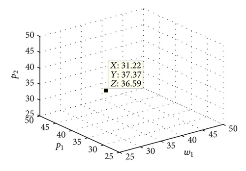
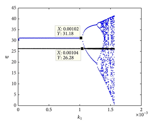
In system (8), letting w_i(t + 1) = w_i(t)(i = 1,2), we can get the fixed points of system (8). Before we solve the fixed points of system (8), we first assign some parameters considering the actual competition: , and . We will calculate all the fixed points and only consider the Nash equilibrium point (w₁ = 31.22, w₂ = 26.33, p₁ = 37.37, and p₂ = 36.59).

Jacobian matrix of (8) in the Nash equilibrium point is

()

Characteristic polynomial of (9) is f(λ) = λ² − Aλ + B, where A = 91895.38k₁ + 119860.3k₂ + 2 and B = 91895.38k₁ + 119860.3k₂ + 10718148142.27k₁k₂ + 1.

The local stability of Nash equilibrium can be gained according to Routh-Hurwiz’s condition:

()

Condition (10) gives the necessary and sufficient conditions of stable region of the Nash equilibrium point. Economic meaning of the stable region is that, whatever initial price is chosen by the two manufacturers in local stable region, they will eventually achieve Nash equilibrium price after finite games. It is important to notice that the two manufacturers may accelerate the price adjustment speed in order to increase their profit. Price adjustment parameter does not change Nash equilibrium point. Once one manufacturer adjusts price too fast and pushes k₁, k₂ out of the stable region, the system tends to become unstable and falls into chaos. On the basis of the parameters assigned above, we use numerical simulation to describe the dynamic behaviors of system (8).

4.2. The Effect of Price Adjustment Speed on the System

(1) The Influence Which the Price Adjustment Speed Has on the Behaviors of the Two Manufacturers and the Retailer. Since the two manufacturers’ behaviors are similar, we only discuss the influence on system behaviors when the parameter of M₁ is changed.

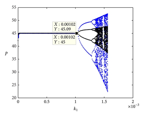
First, we can get the price trajectory diagrams of the two manufacturers and retailer with change of k₁ when k₂ = 0.001, w₁ = 20, and w₂ = 15, as shown in Figure 1(a) and Figure 1(b). We can obtain that w₂ is less affected by change of k₁ and w₁, w₂, p₁, and p₂ change from the stable period, period-doubling bifurcation to the chaos in three trajectories. When k₁ ∈ [0,0.00102], w₁, w₂, p₁, and p₂ are stable. When k₁ = 0.00102, the first bifurcation appears in w₁, w₂, p₁, and p₂, and the price of the two manufacturers and retailer vibrates in two points; after that the second bifurcation appears in the system; finally, the system goes into chaos, the price behaves more disorderly, and the market behaviors become unpredictable. Figure 1(c) shows corresponding change of the Lyapunov exponent. The positive Lyapunov exponent is used to mark the chaos; the bigger the Lyapunov exponent, the stronger the chaos. The system is in chaos when most of the Lyapunov exponents are positive. Figure 2 shows the price trajectory diagrams of the two manufacturers and retailer with the change of k₁ and k₂ simultaneously. We can observe that the stable regions of w₁, w₂ are smaller than the one with change of only k₁ or only k₂ and the w₁, p₁, and p₂ change from the stable period and period-doubling bifurcation to the chaos in four trajectories; the dynamic characteristics of w₂ in particular do not follow the period-doubling bifurcation. Because k₁ and k₂ change at the same time, the retailer’s behaviors appear in complicated characteristics.

Details are in the caption following the image — **Figure 1 (a)**
Open in figure viewer PowerPoint

Price bifurcation and Lyapunov of two manufacturers and retailer with change of k₁ when k₂ = 0.001: (a) wholesale price; (b) retail price; (c) Lyapunov.

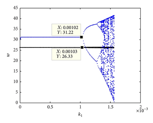
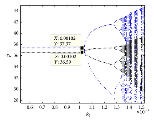
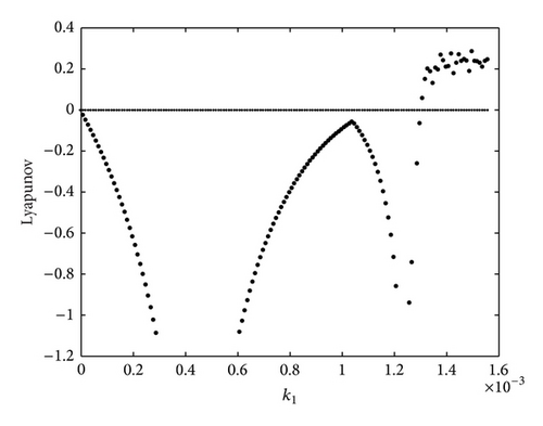
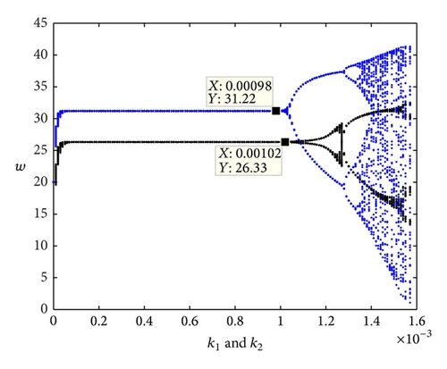
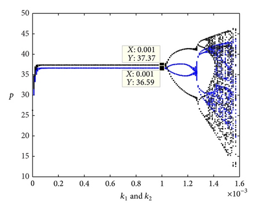
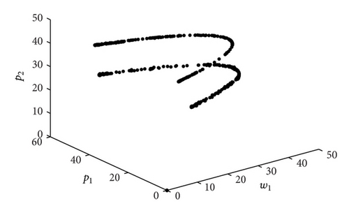
Figure 3(a) shows an attractor of the supply chain which is in stable state when k₁ = k₂ = 0.001. Figure 3(b) shows a chaos attractor of the supply chain which appears in a complex state when k₁ = k₂ = 0.0015; it is another chaos characteristic of the variables.

Proposition 1. The value of price adjustment speed determines whether the supply chain is stable or not; when we determine this value, each manufacturer should consider market reaction of the competitors and retailer. Only upstream and downstream enterprises keep stable, to ensure the stability of the supply chain and to maximize the enterprise’s profit.

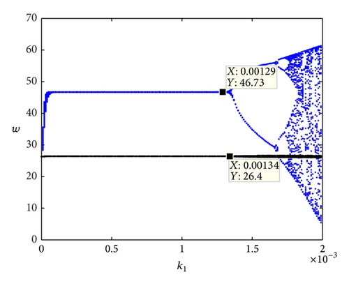
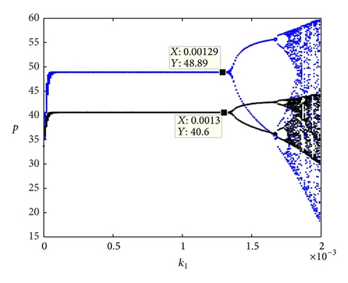
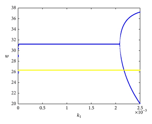
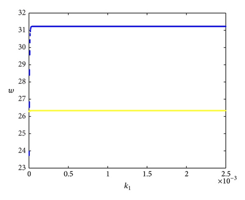
(2) The Influence Which Change of Risk Preference Has on the Behaviors of the Two Manufacturers and the Retailer. Let k₂ = 0.001, R_R = 120; the value of other parameters is the same as in the previous assumption; we can obtain the price bifurcation diagrams of the two manufacturers and the retailer with change of k₁, as shown in Figure 4. We can see that the stable region is not changed, wholesale price of the two manufacturers declines, and the retail price goes up with change of R_R. Figure 5 shows the price bifurcation diagrams of the two manufacturers and the retailer with change of k₁ when , the first bifurcation point is k₁ = 0.00129, and the equilibrium value is (46.73, 26.4, 48.89, and 40.6). We can make a conclusion that the risk preference of the manufacturer can affect the stable region of system and change the equilibrium point of system, and the risk preference of the retailer cannot affect the stable region of system and change the equilibrium point of system.

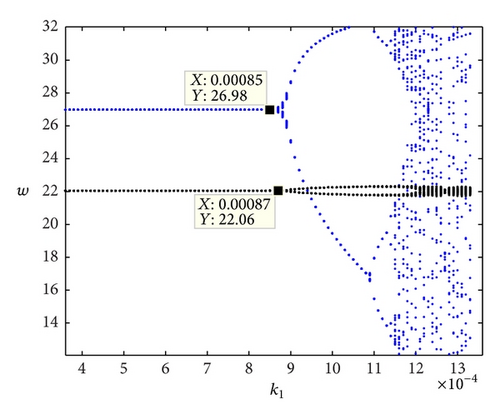
(3) The Influence Which the Uncertain Demand Has on the System Variable Behaviors. Because the demand forecasting exists errors, the customer demand is always uncertain. Next we will observe the price change of the two manufacturers and retailer with change of k₁ when σ = 70, k₂ = 0.001, and it is shown in Figure 6. We can see that, with σ increasing, the first bifurcation point of the system is k₁ = 0.00105, and w₁, w₂, p₁, and p₂ are all falling.

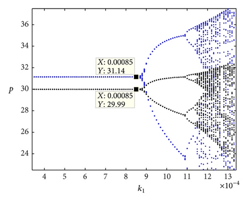
Proposition 2. Uncertain demand makes the supply chain access chaos quickly, and the wholesale price and the retail price decline. It is uncertain about their respective profit; thereby the competitiveness of the supply chain becomes weak.

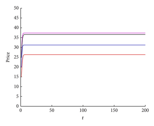
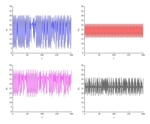
(4) The Power Spectrum of Variables and the Sensitive Dependence on Initial Conditions. We adopt a cycle diagram method to estimate the power spectrum of variables. Next, we will observe the price change of the two manufacturers and retailer when k₁ = k₂ = 0.001 and the initial values are w₁ = 20, w₂ = 15; it is shown in Figure 7. We know that the supply chain is stable when k₁ = k₂ = 0.001, so the power spectrum of the variables is straight lines which conform to the attractor in Figure 3(a). When k₁ = k₂ = 0.0015, the supply chain is in chaos. From Figure 8, we can see that w₁, w₂, p₁, and p₂ vibrate with a frequency, w₂ changes with approximate periodic motion, and range of movement of p₁ is bigger than the one of p₂.

Then, we will observe the price change of the two manufacturers and the retailer when k₁ = k₂ = 0.0015 and (w₁, w₂) = (20.01, 15) and (20, 15) which has smaller change in w₁ and no change in w₂; they are shown in Figure 9. We can see that the price of the two manufacturers and retailer has distinct change. The sensitive dependence on initial conditions is another important characteristic of the chaotic system as it fully manifests the sensitive dependence on the initial conditions of the system (8).

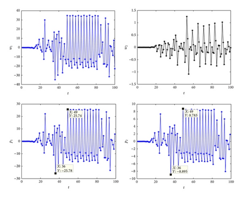
Through the above analysis, we know that the risk-averse supply chain has been in chaos. At this state, the price of the two manufacturers and the retailer changes disorderly from the beginning of the Nash equilibrium.

(5) The Effect of Parameter Change on the Profit. Figure 10 shows the profit bifurcation of the two manufacturers and retailer with changes of k₁. Obviously, the profit bifurcation is similar to price bifurcation including period-doubling bifurcation, four-period-doubling bifurcation, and chaos state. Figure 11 shows the profit of the two manufacturers and retailer in 50 games when the system is in a stationary period, two-period-doubling bifurcation, and a chaotic period. In the different period, the fluctuation range of price of M₁ is larger than that of M₂. Tables 1, 2, and 3 give the profit data of the two manufacturers and retailer, respectively, in different periods with change of , and σ.

Table 1. The profit of the two manufacturers and retailer in different periods when k₁ = 0.001.

Different periods	Stable period	Two-period-doubling bifurcation	Chaotic period
π_R	8159.76	8144.99	8175.85
	8074.74	6126.11	2403.59
	8128.54	8149.99	8054.7

∑ π	24363.04	22421.09	18634.14

Table 2. The profit of the two manufacturers and retailer in different periods when

Different periods	Stable period	Two-period-doubling bifurcation	Chaotic period
π_R	8182.74	8190.65	8203.86
	15539.95	14331.78	12443.96
	8144.84	8136.82	8125.35

∑ π	31867.63	30659.25	28773.17

Table 3. The profit of the two manufacturers and retailer in different periods when σ = 120.

Different periods	Stable period	Two period-doubling bifurcation	Chaotic period
π_R	6001.45	6009.92	6013.69
	5918.76	4346.43	3573.6
	5972.61	5968.58	5967.1

∑ π	17892.81	16324.92	15554.38

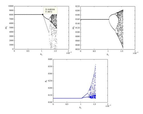
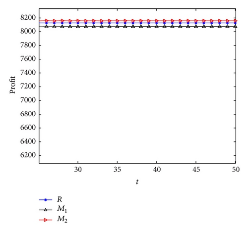
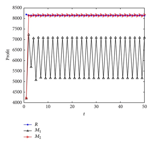
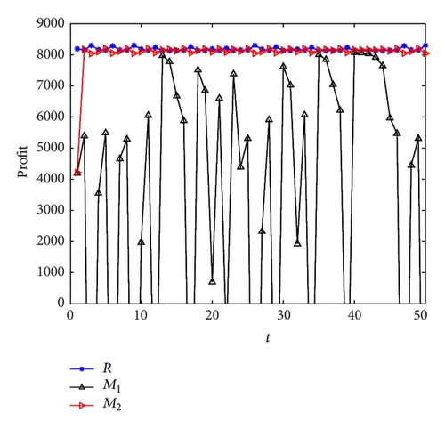
Proposition 3. First, the total profit of the system in the chaotic period is less than that in other periods. Second, the total profit of the system and respective profit of the two manufacturers and the retailer will increase with increase of and decrease with increase of σ. Third, when the system is in chaos, the profit of the two manufacturers will decrease, but the profit of retailer will increase. Namely, when the system goes into chaos, the retailer is a beneficiary. This is why some participants set out contract to avoid disordered competition in some situations and why some participants prefer chaotic market in some cases.

5. Chaos Control

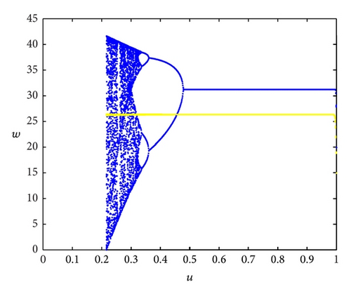
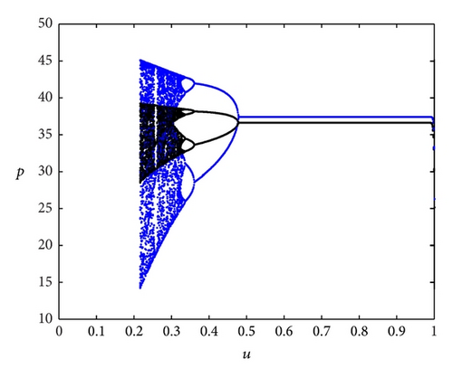
Competitive manufacturers will certainly want to achieve maximum profit in the existing supply chain. Through the above analysis, we can see that the change of k₁, k₂, and σ often causes disorder behaviors in the market which are of disadvantage to the stability of the supply chain and the development of the enterprise. However, the participants often maximize their own profit by any kind of means in the process of marketization. So the market will be out of order and finally falls into chaos. It is particularly important that each participant should make rational strategic decision timely for making the system return to the stable equilibrium.

Parameter adjustment and feedback control method of the system variable will be used to control the chaos of the system (8). It is often used at the chaos control of general discrete dynamic system. We will analyze system chaos control based on the influence of k₁ on the stability of the risk-averse supply chain. Assume system (8) is w_i(t + 1) = f_i(w₁(t), w₂(t)); the system under control is as follows:

()

When u = 0, the controlled system is the original system; thus, the controlled system has the same periodic orbit a the original system. When m = 1, each step iteration of the fixed point is in control. When m = 2, 4, and so forth, namely, to control the second cycle orbit, four cycles orbit. As long as we select an appropriate value for u, we can ensure delayed bifurcation with k₁ at fixed point and keep the supply chain being stable within large scope of k₁. In addition, with appropriate adjustment value of m, we can realize stability control of higher cycle orbits for the chaotic attractor. Then, we discuss the stability control in the supply chain when m = 1 and try to stabilize the price on the fixed point. The controlled system can be represented as

()

Figures 12 and 13 show that the chaos system can be controlled gradually from the four-period-doubling bifurcation and two-period-doubling bifurcation to the fixed point with the control parameter u increasing. When u > 0.4825, the controlled system can be stabilized at the Nash equilibrium point. In a real market, we can consider u as the regulation on the price adjustment speed which could avoid market chaos when manufacturers pursue their maximum profit. We can also consider u as the learning ability or adaptability of the market. For instance, the manufacturer will adjust price according to the information in the past. Due to the complexity, disorder, and randomness in chaotic state, the manufacturer should have a clear forecast of chaos control. After adjusting parameter u, we can make the periodic orbit stable at the expected point.

6. Conclusions

Considering the randomness of customer’s requirements and supply’s risk preference, we study the supply chain in the market which consists of two manufacturers and a retailer. We construct a dynamic Stackelberg and Bertrand pricing game model and find that bifurcation, chaos, and other complex phenomena occur when the price adjustment speed, the level of risk preference, and predict error change. When the chaos occurs, the stability of the whole supply system is broken, and the market becomes abnormal, irregular, and unpredictable. It is important to note that, when determining the value of the parameter, each manufacturer should consider the market reaction of competitors and retailer to ensure that the upstream and downstream enterprises keep stable and ensure that the supply chain keeps stable for their maximum profit. Finally, we use the parameter adjustment method to control the supply system. Then, we have obtained some conclusions from our research.

(1)
The two manufacturers play the Bertrand game; when M₁ changes its price adjustment speed, its wholesale price presents deterministic characteristics of chaos, and the wholesale price of M₂ is influenced less. The price of retailer is influenced largely. When price adjustment speed of the two manufacturers changes at the same time, it has no effect on the optimal pricing strategy, the stable region of the supply chain gets smaller, and the two manufacturers all show complicated behavior characteristics.
(2)
Increasing the risk tolerance level of the retailer does not impact stable region, but retail price will increase and wholesale price of the two manufacturers will fall. If M₁ increases his risk tolerance level, the stability between M₁ and the retailer is enhanced, and the two manufacturers’ wholesale price and products’ retail price go up. Uncertain demand makes the wholesale prices and retailer prices access chaos quickly, two manufacturers’ wholesale price and retail price decline, and total profit and their respective profit decrease.
(3)
The total profit of the system in the chaotic period is less than that in other periods; it and respective profit of the two manufacturers and the retailer will increase with increase of and decrease with increase of σ. When the system is in chaos, the profit of the two manufacturers will decrease, but the profit of retailer will increase. Namely, when the system goes into the chaos, the weaker (retailer) is a beneficiary.

This paper is a realistic guide for the risk-averse supply chain to formulate its parameter adjustment strategies to avoid the loss of the respective profit and the total profit. It is also a realistic reference for the managers to formulate relevant policies on macroeconomic control. The managers can adjust parameters to make the supply chain in good operating condition based on the operation condition of the supply chain; for example, when the variance of customer demand gets bigger, the manager should reduce the price adjustment speed for the stability of the supply chain.

There are several possible directions for the future study. First, one can study three-echelon supply chain with complexity behaviors under the different game strategies considering the delay time, such as the Stackelberg game between the two manufacturers. Second, one can adopt a different form of demand function and, finally, other control methods may be applied in order to achieve different results.

Conflict of Interests

The authors declare that there is no conflict of interests regarding the publication of this paper.

Acknowledgments

The authors thank the reviewers for their careful reading and providing some pertinent suggestions. The research was supported by the National Natural Science Foundation of China (No. 61273231), Doctoral Fund of Ministry of Education of China (Grant No. 20130032110073) and supported by Tianjin University Innovation Fund.

References

1 Wei J., Zhao J., and Li Y., Pricing decisions for complementary products with firms′ different market powers, European Journal of Operational Research. (2013) 224, no. 3, 507–519, https://doi.org/10.1016/j.ejor.2012.09.011, MR2992261.
10.1016/j.ejor.2012.09.011
Web of Science® Google Scholar
2 Mukhopadhyay S. K., Yue X., and Zhu X., A Stackelberg model of pricing of complementary goods under information asymmetry, International Journal of Production Economics. (2011) 134, no. 2, 424–433, 2-s2.0-80052393165, https://doi.org/10.1016/j.ijpe.2009.11.015.
10.1016/j.ijpe.2009.11.015
Web of Science® Google Scholar
3 Caliskan-Demirag O., Chen Y., and Li J., Customer and retailer rebates under risk aversion, International Journal of Production Economics. (2011) 133, no. 2, 736–750, 2-s2.0-80051550583, https://doi.org/10.1016/j.ijpe.2011.06.002.
10.1016/j.ijpe.2011.06.002
Web of Science® Google Scholar
4 Luo C. and Huang J., Pricing and ordering strategies in supply chain with different risk preference, Computer Integrated Manufacturing Systems. (2012) 18, no. 4, 859–866.
Google Scholar
5 Hu B. and Chen X., Supply chain sale-surety option contract with effort dependent demand and risk preference, Journal of Industrial Engineering: Engineering Management. (2012) 26, no. 3, 184–190.
Google Scholar
6 Guan Z. and Zhou B., Integrated optimization of three-level supply chain under different risk attitude, Operations Research and Management Science. (2011) 20, no. 6, 19–24.
Google Scholar
7 Huang S. and Yang C., Supply chain coordination model considering risk attitudes of agents with VaR constraints, Journal of Industrial Engineering: Engineering Management. (2012) 25, no. 2, 136–141.
Google Scholar
8 Puu T., The chaotic duopolists revisited, Journal of Economic Behavior and Organization. (1998) 33, no. 3-4, 385–394, 2-s2.0-0032517943, https://doi.org/10.1016/S0167-2681(97)00064-4.
10.1016/S0167-2681(97)00064-4
Web of Science® Google Scholar
9 Ma J. and Sun Z., The research on price game model and its complex characteristics of triopoly in different decision-making rule, Nonlinear Dynamics. (2013) 71, no. 1-2, 35–53, https://doi.org/10.1007/s11071-012-0640-7, MR3010562.
10.1007/s11071-012-0640-7
Web of Science® Google Scholar
10 Ma J. and Bangura H. I., Complexity analysis research of financial and economic system under the condition of three parameters′ change circumstances, Nonlinear Dynamics. (2012) 70, no. 4, 2313–2326, https://doi.org/10.1007/s11071-012-0336-z, MR2998164, ZBL1268.34084.
10.1007/s11071-012-0336-z
Web of Science® Google Scholar
11 Hwarng H. B. and Xie N., Understanding supply chain dynamics: a chaos perspective, European Journal of Operational Research. (2008) 184, no. 3, 1163–1178, 2-s2.0-34548571914, https://doi.org/10.1016/j.ejor.2006.12.014, ZBL1141.90444.
10.1016/j.ejor.2006.12.014
Web of Science® Google Scholar
12 Wang J. and Wang X., Complex dynamic behaviors of constrained supply chain systems, Systems Engineering-Theory & Practice. (2012) 32, no. 4, 746–751.
Google Scholar
13 Ma J. and Feng Y., The study of the chaotic behavior in retailer′s demand model, Discrete Dynamics in Nature and Society. (2008) 2008, 12, 792031, https://doi.org/10.1155/2008/792031, MR2465501, ZBL1158.91419.
10.1155/2008/792031
Web of Science® Google Scholar
14 Gal-Or E., Information sharing in oligopoly, Econometrica. (1985) 53, no. 2, 329–343, https://doi.org/10.2307/1911239, MR785472, ZBL0578.90008.
10.2307/1911239
Web of Science® Google Scholar
15 Raju J. S. and Roy A., Market information and firm performance, Management Science. (2000) 46, no. 8, 1075–1084, 2-s2.0-0034249426, https://doi.org/10.1287/mnsc.46.8.1075.12024, ZBL1232.91444.
10.1287/mnsc.46.8.1075.12024
Web of Science® Google Scholar
16 Vives X., Duopoly information equilibrium: cournot and Bertrand, Journal of Economic Theory. (1984) 34, no. 1, 71–94, https://doi.org/10.1016/0022-0531(84)90162-5, MR765787, ZBL0546.90011.
10.1016/0022-0531(84)90162-5
Web of Science® Google Scholar
17 Kunstman A., Decision making under uncertainty: models and choices, European Journal of Operational Research. (1981) 8, no. 4, 401–402.
10.1016/0377-2217(81)90014-X
Web of Science® Google Scholar
18 Walls M. R., Combining decision analysis and portfolio management to improve project selection in the exploration and production firm, Journal of Petroleum Science and Engineering. (2004) 44, no. 1-2, 55–65, 2-s2.0-6444225911, https://doi.org/10.1016/j.petrol.2004.02.005.
10.1016/j.petrol.2004.02.005
CAS Web of Science® Google Scholar
19 Banker R. D., Khosla I., and Sinha K. K., Quality and competition, Management Science. (1998) 44, no. 9, 1179–1192, 2-s2.0-0032154238, https://doi.org/10.1287/mnsc.44.9.1179, ZBL0989.91538.
10.1287/mnsc.44.9.1179
Web of Science® Google Scholar

Citing Literature

All articles

The Complex Dynamics of Bertrand-Stackelberg Pricing Models in a Risk-Averse Supply Chain

Abstract

1. Introduction