Volume 2014, Issue 1 628357

Research Article

Open Access

Particle Swarm Optimization Based on Local Attractors of Ordinary Differential Equation System

Wenyu Yang,

Wenyu Yang

College of Science, Huazhong Agricultural University, Wuhan 430070, China hzau.edu.cn

Search for more papers by this author

Wei Wu,

Corresponding Author

Wei Wu

[email protected]

School of Mathematical Sciences, Dalian University of Technology, Dalian 116024, China dlut.edu.cn

Search for more papers by this author

Yetian Fan,

Yetian Fan

School of Mathematical Sciences, Dalian University of Technology, Dalian 116024, China dlut.edu.cn

Search for more papers by this author

Zhengxue Li,

Zhengxue Li

School of Mathematical Sciences, Dalian University of Technology, Dalian 116024, China dlut.edu.cn

Search for more papers by this author

Wenyu Yang,

Wenyu Yang

College of Science, Huazhong Agricultural University, Wuhan 430070, China hzau.edu.cn

Search for more papers by this author

Wei Wu,

Corresponding Author

Wei Wu

[email protected]

School of Mathematical Sciences, Dalian University of Technology, Dalian 116024, China dlut.edu.cn

Search for more papers by this author

Yetian Fan,

Yetian Fan

School of Mathematical Sciences, Dalian University of Technology, Dalian 116024, China dlut.edu.cn

Search for more papers by this author

Zhengxue Li,

Zhengxue Li

School of Mathematical Sciences, Dalian University of Technology, Dalian 116024, China dlut.edu.cn

Search for more papers by this author

First published: 26 August 2014

https://doi.org/10.1155/2014/628357

Citations: 3

Academic Editor: Manuel De la Sen

Share a link

Email
Wechat
Bluesky

Abstract

Particle swarm optimization (PSO) is inspired by sociological behavior. In this paper, we interpret PSO as a finite difference scheme for solving a system of stochastic ordinary differential equations (SODE). In this framework, the position points of the swarm converge to an equilibrium point of the SODE and the local attractors, which are easily defined by the present position points, also converge to the global attractor. Inspired by this observation, we propose a class of modified PSO iteration methods (MPSO) based on local attractors of the SODE. The idea of MPSO is to choose the next update state near the present local attractor, rather than the present position point as in the original PSO, according to a given probability density function. In particular, the quantum-behaved particle swarm optimization method turns out to be a special case of MPSO by taking a special probability density function. The MPSO methods with six different probability density functions are tested on a few benchmark problems. These MPSO methods behave differently for different problems. Thus, our framework not only gives an interpretation for the ordinary PSO but also, more importantly, provides a warehouse of PSO-like methods to choose from for solving different practical problems.

1. Introduction

Inspired by sociological behavior associated with bird flock, particle swarm optimization (PSO) was first introduced by Kennedy and Eberhart [1]. In a PSO, the individual particles of a swarm fly stochastically toward the positions of their own previous best performance and the best previous performance of the swarm. Researchers have been trying to excogitate new framework to interpret PSO in order to analyze the property of PSO and to construct new PSO-like methods. For instance, in [2] PSO is interpreted as a difference scheme for a second-order ordinary differential equation. Fernández-Martínez et al. interpret PSO algorithm as a stochastic damped mass-spring system: the so-called PSO continuous model and present a theoretical analysis of PSO trajectories in [3]. Based on a continuous vesion of PSO, Fernández Martínez and García Gonzalo propose Generalized PSO(GPSO) in [4] and introduce a delayed version of the PSO continuous model in [5]. Furthermore, Fernández-Martínez and García-Gonzalo give stochastic stability analysis of PSO models in [6] and propose two novel algorithms: PP-GPSO and RR-GPSO in [7]. PSO algorithms have been applied successfully for practical applications [8–10].

In [11], a so-called quantum-behaved particle swarm optimization (QPSO) is proposed based on an assumption that the individual particles in a PSO system have quantum behavior. A wide range of continuous optimization problems have been solved successfully by QPSO and many efficient strategies have been proposed to improve the algorithm [11–20]. A global convergence analysis of QPSO is given by Sun et al. in [21].

In this paper, we interpret PSO as a finite difference scheme for solving a system of stochastic ordinary differential equations (SODE in short). In this framework, the convergent point of the position points in the PSO iteration process corresponds to an equilibrium point (a global attractor) of the SODE. We observe that the local attractors, which are easily computed by using the present position points, also converge to the global attractor in the PSO iteration process. Inspired by this observation, we propose a class of modified PSO iteration methods (MPSO in short) based on local attractors of the SODE. The idea of MPSO is to choose the next update state in a neighbourhood of the present local attractor, rather than the present position point as in the original PSO, according to a given probability density function. We will test the MPSO methods with six different probability density functions for solving a few benchmark problems. These MPSO methods behave differently for different problems. Thus, our framework not only gives an interpretation for the ordinary PSO but also, more importantly, provides a warehouse of PSO-like methods to choose from for solving different practical problems.

Our work is partly inspired by the second-order ordinary differential equation framework for PSO in [2, 3]. But the solution of a second-order ordinary differential equation is somehow more difficult to describe and it seems more difficult to construct new PSO-like methods through this framework. Our framework of ordinary differential equation makes the job easier.

Our work is also inspired by the quantum-behaved particle swarm optimization (QPSO) method in [11]. It turns out that QPSO becomes a special case of our MPSO by choosing a special probability density function. And fortunately, the convergence analysis for QPSO given in [21] is still valid for our MPSO methods. In fact, what matters in the convergence analysis is a suitable choice of the probability density function, and the particular quantum behavior does nothing in the convergence analysis.

The rest of the paper is organized as follows. In Section 2 we interpret PSO as a system of ODE and propose a class of MPSO methods. Then, in Section 3 we test, on some nonlinear benchmark functions, our MPSO methods with different probability density functions. Finally, some conclusions are gathered in Section 4.

2. Particle Swarm Optimization Algorithms

2.1. The Original PSO

Particle swarm optimization algorithm (PSO) was first introduced in Kennedy and Eberhart [1] inspired by sociological behavior associated with bird flock. In a PSO with population size M, the velocity vector V and the position vector X of each particle are iteratively adjusted to minimize an R^N → R objective function f with X as input value. At the nth iteration step, the particle i updates its velocity vector

and position vector

according to

()

for n = 1,2, … and 1 ≤ j ≤ N, where

and

are random numbers uniformly distributed on (0,1). The values of

and

are scaled by the constants c₁ and c₂ which are called acceleration coefficients. The vector

denotes the personal best position (pbest in short), which is the position of particle i giving the best objective function value so far, and the vector

is the global best (gbest) position which is the position of the best particle among all particles. They are updated according to

()

When the PSO system is convergent, all particles converge, as n tends to infinity, to a global attractor G^*; that is,

()

and their velocity vectors V_i,n converge to zero.

2.2. Interpretation of PSO as a Finite Difference Scheme for an SODE

Let us rewrite the iteration formula (1) for PSO as a system of difference equations:

()

for t = 1,2, …, where

()

Generally but not necessarily, the constants c₁ and c₂ are set to be equal. For the sake of simple representation, we rewrite

()

where

. We regard (4) as a finite difference scheme with time step length Δt = 1 for solving the following system of stochastic ordinary differential equations (SODE):

()

where 1 ≤ i ≤ M, 1 ≤ j ≤ N,

, and

for all real numbers t > 0. Let

, and

, where

, and so forth. Then, the SODE (7) is written as

()

where g is a nonlinear function. The theoretical analysis of this SODE and its difference schemes is difficult, but it is not our concern. For our purpose, we recall that usually, or at least very often, the solution of a difference scheme for an ODE will converge to an equilibrium point Z^* satisfying g(Z^*) = 0 when the iteration time n tends to infinity. Thus, the convergent point of the PSO iteration process corresponds to an equilibrium point of the SODE.

Usually, for an equilibrium point Z^* = (V^*, X^*) of the SODE (7) we have

()

for some constant vector l^* ∈ R^N. Let us call

the local attractor and X^* the global attractor for the SODE at time t.

2.3. MPSO for Iteratively Decreasing

Now, let us forget the original PSO and concentrate on the task of finding a global attractor (an equilibrium point) of the SODE (7). Based on (10), we see that finding an equilibrium point of the ODE system (7) is equivalent to making the position vector closer and closer to the local attractor . Thus, we choose the next update state in a neighbourhood of the present local attractor, rather than the present position point as in the original PSO, according to a given probability density function (PDF).

Define

()

where α is an adjustable parameter and

is the mbest position defined by the average of the pbest positions of all particles; that is,

. We choose a PDF Q(Y; L) using

as a parameter indicating the “width" of the support of the function. Choose a random number

, according to the PDF

. Then, the update formula of MPSO is as follows:

()

where the signs + and − are taken randomly in equal probability and

. p_n = (p_1,n, p_2,n, …, p_M,n), a discrete approximation of the local attractor

, is called discrete local attractor at nth step. Therefore, X_n+1 = (X_1,n+1, X_2,n+1, …, X_M,n+1) is a point randomly chosen from a neighborhood of the discrete local attractor p_n.

Our MPSO algorithm is described in detail in Algorithm 1.

Algorithm 1

Choose a PDF Q(Y; L).
Initialize population position vector X
Do
For i = 1 to population size M
If f(X_i) < f(P_i) Then P_i = X_i
End For
For i = 1 to population size M
For j = 1 to dimension N
Choose α and compute .
Choose a random number ,
according to the PDF .
Choose , .
If rand(0,1) > 0.5 Then
If rand(0,1) < 0.5 Then
End For
End For
Repeat the iteration until all the increments are small enough
or some other termination criterion is satisfied.

2.3.1. MPSO with Different PDFs

As examples, we give six different PDFs and depict them when

in Figures 1, 2, 3, 4, 5, and 6.

()

Details are in the caption following the image — **Figure 1**
Open in figure viewer PowerPoint

Figure of the probability density function Q₁.

Now, let us demonstrate how to choose a random number

according to the probability density function

. First, we obtain the corresponding probability distribution function F(Y) by

()

Then, for a randomly given number

, we solve the equation

()

to get

()

Therefore, the update formulas corresponding to Q₁–Q₆ can be written as follows:

()

where u ~ U(0,1), u₁ ~ U(0,1), and u₂ ~ U(0,1). Here the superscripts and subscripts of X and L have been removed for the sake of clear representation. For instance, in the case of Q₅, the precise formula is

()

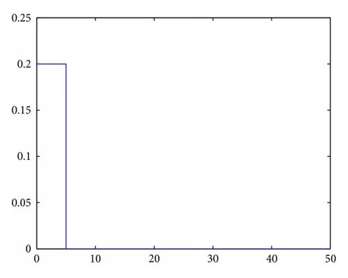
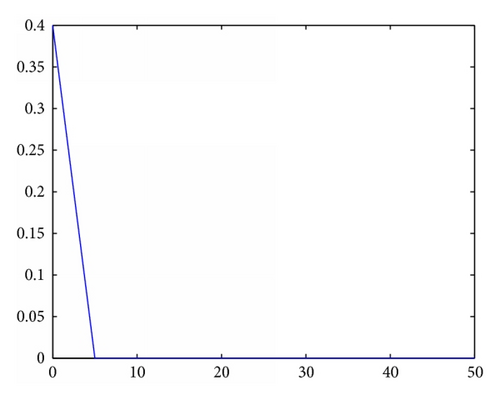
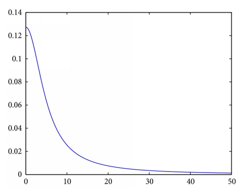
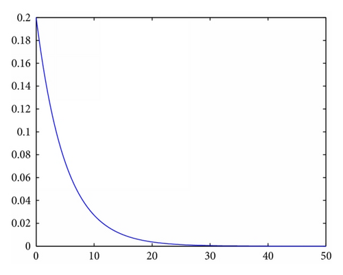
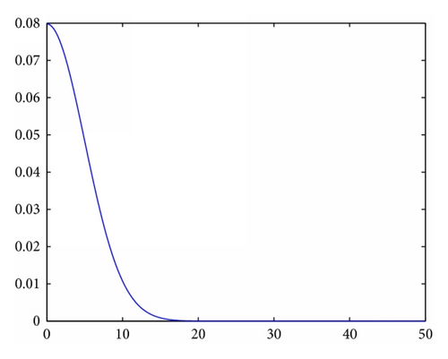
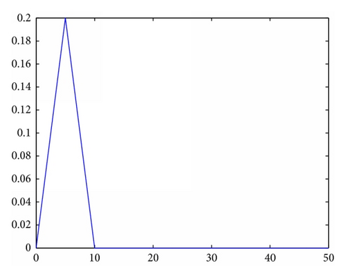
2.4. Quantum-Behaved Particle Swarm Optimization

In QPSO proposed by Sun et al. [11], the quantum state of a particle is depicted by a wave function

, which is the solution of the Schrödinger equation

()

where Hamiltonian operator is

()

Note that the Schrödinger equation is a second-order partial differential equation. |Ψ|² is chosen to be the PDF for the present position of the particle. In particular, Q₅ and Q₆ defined above are two such PDFs mentioned in [11]. Thus, QPSO can be regarded as a special case of MPSO. But the other four PDFs Q₁ to Q₄ are not related to the Schrödinger equation.

Let us elaborate a little bit on QPSO. In [11], Sun et al. assume that, at the nth iteration, on the jth dimension (1 ≤ j ≤ N) of the search space, particle i moves in a δ potential well centered at which is the jth dimension coordinate of its local attractor.

Let

, then they obtained the PDF

()

in Jun Sun et al. [17] is determined by

()

where

is the mbest position. Finally,

()

Sun et al. gave a global convergence analysis of QPSO in [20], which employed certain properties of the PDF but had nothing to do with the particular Schördinger equation. Actually, all our six PDFs given Section 2.3.1 possess these properties, and hence the global convergence analysis applies.

3. Numerical Simulation

In this section, we use MPSO with six different PDFs mentioned in Section 2 to test five nonlinear benchmark functions used in [11]. The first function is the Sphere function described by

()

The second function is Rosenbrock function described by

()

The third function is the generalized Rastrigrin function described by

()

The fourth function is the generalized Griewank function described by

()

The last function is Shcaffer function described by

()

where x = (x₁, x₂, …, x_n) is an n-dimension real-valued vector. The initialization and search ranges of the four functions used in [11] are listed in Table 1.

Table 1. Asymmetric initialization and search ranges.

Function	Asymmetric initialization range	Search range
Sphere	(50,100) ⁿ	[−100,100] ⁿ
Rosenbrock	(15,30) ⁿ	[−100,100] ⁿ
Genralized Rastrigrin	(2.56,5.12) ⁿ	[−10,10] ⁿ
Genralized Griewank	(300,600) ⁿ	[−600,600] ⁿ
Schaffer	(30,100) ⁿ	[−100,100] ⁿ

As in [11], different population sizes (20, 40, and 80) are used for each function to investigate the scalability. The maximum number of the generations is set to 1000, 1500, and 2000, corresponding to the dimensions 10, 20, and 30 for the four functions, respectively. The mean best fitness values and standard deviations, out of total 50 runs of MPSO with different PDFs on f₁ to f₅, are shown in Tables 2, 3, 4, 5, and 6. In the tables, α is the parameter in (12), and α = 1 → 0.5 means that α decreases linearly from 1 to 0.5. The boldface results are obtained by performing the QPSO algorithm in [11], which is equivalent to MPSO with the PDF Q₅. An efficiency comparison of MPSOs with different PDFs on f₁ to f₅ is presented in Table 7.

Table 2. Mean best fitness values and standard deviation for the sphere function.

PDF	Dim.	G_max⁡	M = 20		M = 40		M = 80
PDF	Dim.	G_max⁡	Mean best	Standard deviation	Mean best	Standard deviation	Mean best	Standard deviation
Q₁ (α = 2 → 1.6)	10	1000	9.76E − 25	1.77E − 24	1.31E − 27	7.55E − 27	2.58E − 30	1.70E − 29
	20	1500	9.71E − 13	2.71E − 12	2.26E − 16	4.45E − 16	1.18E − 20	2.35E − 20
	30	2000	8.36E − 07	1.21E − 06	2.65E − 09	3.76E − 09	1.59E − 12	2.94E − 12

Q₂ (α = 2.5 → 2)	10	1000	1.24E − 32	8.66E − 32	3.32E − 62	2.14E − 61	9.67E − 88	4.14E − 87
	20	1500	3.16E − 17	2.21E − 16	1.96E − 35	1.35E − 34	4.82E − 50	2.78E − 49
	30	2000	4.15E − 12	1.99E − 11	1.24E − 24	5.66E − 24	3.57E − 36	2.32E − 35

Q₃ (α = 2 → 1.2)	10	1000	4.36E − 19	1.77E − 18	4.05E − 28	2.83E − 27	7.77E − 40	5.41E − 39
	20	1500	1.28E − 08	4.99E − 08	1.07E − 15	3.57E − 15	2.86E − 22	1.20E − 21
	30	2000	4.69E − 05	1.06E − 04	4.73E − 10	9.70E − 10	2.58E − 14	9.63E − 14

Q₄ (α = 0.5 → 0.25)	10	1000	9.65E − 24	6.65E − 23	8.46E − 38	5.87E − 37	1.47E − 49	7.85E − 49
	20	1500	7.37E − 14	4.02E − 13	3.33E − 22	6.45E − 22	4.30E − 29	1.27E − 28
	30	2000	1.31E − 07	5.47E − 07	2.58E − 10	1.80E − 09	3.76E − 18	1.20E − 17

Q₅ (α = 1 → 0.5)	10	1000	1.18E − 27	6.19E − 27	8.47E − 40	5.82E − 39	8.09E − 53	5.23E − 52
	20	1500	1.16E − 14	4.48E − 14	1.47E − 23	7.46E − 23	1.04E − 31	3.46E − 31
	30	2000	7.16E − 09	4.01E − 08	2.73E − 16	6.02E − 16	9.68E − 22	3.07E − 21

Q₆ (α = 1.2 → 0.8)	10	1000	1.98E − 29	1.39E − 28	3.91E − 51	2.56E − 50	1.24E − 64	8.50E − 64
	20	1500	4.43E − 18	1.43E − 17	2.23E − 28	6.62E − 28	2.37E − 38	9.78E − 38
	30	2000	2.82E − 11	1.06E − 10	2.12E − 19	8.70E − 19	1.31E − 26	4.29E − 26

Table 3. Mean best fitness values and standard deviation for the Rosenbrock function.

PDF	Dim.	G_max⁡	M = 20		M = 40		M = 80
PDF	Dim.	G_max⁡	Mean best	Standard deviation	Mean best	Standard deviation	Mean best	St andard deviation
Q₁ (α = 2 → 1.6)	10	1000	17.9685	29.8452	12.2590	21.7814	11.7597	26.2940
	20	1500	111.6378	188.7111	60.2500	50.6469	46.2081	41.0317
	30	2000	416.5972	1436.0	112.4362	145.4795	72.8064	99.0574

Q₂ (α = 2.5 → 2)	10	1000	33.6155	49.8280	26.2646	43.4507	8.2692	9.3772
	20	1500	82.0246	67.5004	60.3972	51.3739	44.3745	42.1392
	30	2000	138.9158	138.7761	83.9015	80.3806	68.5438	42.1898

Q₃ (α = 2 → 1.6)	10	1000	17.2888	36.1287	16.5371	31.0729	11.9782	26.6798
	20	1500	89.6570	162.4040	54.0191	56.6993	49.7047	50.1423
	30	2000	221.5118	539.5228	86.1085	152.8715	67.2254	103.1385

Q₄ (α = 0.5 → 0.25)	10	1000	71.5892	150.1641	29.8696	46.9684	17.7129	18.4078
	20	1500	86.1848	107.0572	78.7056	95.2644	52.9101	47.3649
	30	2000	154.0989	203.9596	104.0223	155.8188	80.6434	88.6188

Q₅ (α = 1 → 0.5)	10	1000	45.6945	93.5950	14.9285	18.8043	9.2944	12.6001
	20	1500	120.3651	166.2435	77.0110	96.0561	57.0820	45.8037
	30	2000	242.7943	408.3627	135.5536	204.6100	56.0855	45.8168

Q₆ (α = 1.2 → 0.6)	10	1000	20.5409	30.0800	14.8070	21.2420	10.4618	20.9702
	20	1500	93.9863	127.0970	86.2331	129.4297	49.4717	51.3767
	30	2000	504.8399	1090.4	145.6577	198.6213	80.3452	53.4474

Table 4. Mean best fitness values and standard deviation for the generalized Rastrigrin function.

PDF	Dim.	G_max⁡	M = 20		M = 40		M = 80
PDF	Dim.	G_max⁡	Mean best	Standard deviation	Mean best	Standard deviation	Mean best	Standard deviation
Q₁ (α = 2 → 1.2)	10	1000	5.8080	4.0212	4.1037	3.3882	3.1426	3.0072
	20	1500	14.9072	4.9084	10.1125	3.1486	7.5353	2.4052
	30	2000	31.5566	7.7407	20.4983	4.8202	14.4129	3.1085

Q₂ (α = 2.5 → 2)	10	1000	9.9946	5.2287	5.9174	3.0855	4.5410	2.3456
	20	1500	25.7827	10.8980	19.7675	8.6651	15.2177	5.7206
	30	2000	44.8329	14.6816	28.6026	8.0842	23.8493	10.6089

Q₃ (α = 2 → 1.2)	10	1000	4.9402	3.6175	3.0414	3.2103	1.8484	1.1974
	20	1500	15.7036	4.8358	9.6034	2.6184	7.8317	2.4439
	30	2000	31.3558	7.7029	18.3678	4.8567	14.8082	3.2635

Q₄ (α = 0.5 → 0.1)	10	1000	4.5903	2.4440	2.6680	1.5771	2.1146	1.3227
	20	1500	15.2589	5.9192	11.4040	4.5605	9.1622	4.9490
	30	2000	31.5361	12.5203	22.5729	10.0456	17.8487	8.0797

Q₅ (α = 1 → 0.5)	10	1000	6.4976	3.9073	3.0799	1.6581	2.6277	1.5756
	20	1500	16.3392	6.5859	10.7055	3.4636	9.8460	3.6358
	30	2000	32.8285	11.4557	23.2707	7.5592	16.1005	3.5702

Q₆ (α = 1.2 → 0.6)	10	1000	5.4773	4.4511	3.4689	1.8336	2.4370	1.3997
	20	1500	16.2287	5.2804	10.9497	3.1922	8.7061	2.8914
	30	2000	35.3445	9.7132	22.2326	5.6518	18.6051	5.6434

Table 5. Mean best fitness values and standard deviation for the generalized Griewank function.

PDF	Dim.	G_max⁡	M = 20		M = 40		M = 80
PDF	Dim.	G_max⁡	Mean best	Standard deviation	Mean best	Standard deviation	Mean best	Standard deviation
Q₁ (α = 2 → 1.2)	10	1000	0.0846	0.1467	4.49E − 05	2.44E − 04	3.01E − 07	1.82E − 06
	20	1500	0.0049	0.0240	3.24E − 08	1.38E − 07	5.16E − 07	3.61E − 06
	30	2000	0.0024	0.0094	3.09E − 06	1.29E − 05	2.64E − 08	1.69E − 07

Q₂ (α = 2.5 → 2)	10	1000	0.0531	0.0951	3.66E − 06	1.59E − 05	3.06E − 07	1.69E − 06
	20	1500	2.59E − 08	9.64E − 08	2.50E − 09	1.74E − 08	0	0
	30	2000	2.15E − 06	1.33E − 05	1.94E − 11	1.35E − 10	0	0

Q₃ (α = 2 → 1.2)	10	1000	0.0548	0.1063	6.05E − 06	2.53E − 05	6.90E − 08	4.05E − 07
	20	1500	0.0013	0.0072	9.13E − 08	3.23E − 07	1.06E − 08	6.13E − 08
	30	2000	0.0054	0.0096	2.76E − 05	6.40E − 05	1.78E − 08	4.73E − 08

Q₄ (α = 0.5 → 0.1)	10	1000	0.0748	0.1122	1.75E − 05	9.24E − 05	4.63E − 08	1.73E − 07
	20	1500	0.0051	0.0174	1.78E − 08	6.47E − 08	3.98E − 10	1.97E − 09
	30	2000	7.77E − 06	1.72E − 05	4.08E − 09	1.32E − 08	4.27E − 09	2.95E − 08

Q₅ (α = 1 → 0.5)	10	1000	0.0362	0.0553	0.0010	0.0072	4.36E − 08	2.40E − 07
	20	1500	0.0022	0.0097	9.19E − 08	6.36E − 07	3.40E − 09	2.24E − 08
	30	2000	5.61E − 05	1.16E − 04	5.80E − 08	1.33E − 07	6.33E − 07	4.40E − 06

Q₆ (α = 1.2 → 0.6)	10	1000	0.0452	0.0837	0.0092	0.0647	1.97E − 07	8.15E − 07
	20	1500	0.0055	0.0190	3.26E − 07	1.25E − 06	2.11E − 10	1.08E − 09
	30	2000	0.0012	0.0056	1.89E − 06	4.10E − 06	2.07E − 08	9.23E − 08

Table 6. Mean best fitness values and standard deviation for the Schaffer function.

PDF	Dim.	G_max⁡	M = 20		M = 40		M = 80
PDF	Dim.	G_max⁡	Mean best	Standard deviation	Mean best	Standard deviation	Mean best	Standard deviation
Q₁ (α = 2 → 1)	2	1000	5.86E − 04	0.0023	1.04E − 06	2.14E − 06	1.27E − 07	3.16E − 07
	2	1500	7.79E − 04	0.0026	6.89E − 07	3.93E − 06	1.86E − 08	5.16E − 08
	2	2000	7.80E − 04	0.0026	2.53E − 08	7.53E − 08	5.04E − 09	9.42E − 09

Q₂ (α = 2.5 → 2)	2	1000	0.0068	0.0045	0.0047	0.0049	9.23E − 04	0.0029
	2	1500	0.0064	0.0046	0.0033	0.0046	0.0014	0.0034
	2	2000	0.0075	0.0016	0.0033	0.0046	0.0019	0.0039

Q₃ (α = 1 → 0.25)	2	1000	1.00E − 04	0.0029	1.12E − 05	3.92E − 05	6.55E − 07	1.78E − 06
	2	1500	3.22E − 06	5.55E − 06	6.36E − 07	1.23E − 06	1.17E − 07	3.49E − 07
	2	2000	2.00E − 06	6.11E − 06	2.72E − 07	8.83E − 07	1.65E − 08	2.26E − 08

Q₄ (α = 1.2 → 0.6)	2	1000	6.02E − 04	0.0023	3.09E − 06	1.52E − 05	3.41E − 07	9.90E − 07
	2	1500	7.80E − 04	0.0026	4.63E − 06	2.87E − 05	3.35E − 08	1.10E − 07
	2	2000	1.94E − 04	0.0014	4.64E − 08	1.37E − 07	1.16E − 08	2.98E − 08

Q₅ (α = 1.2 → 0.5)	2	1000	0.0023	0.0041	2.05E − 04	0.0014	5.85E − 07	1.62E − 06
	2	1500	9.73E − 04	0.0029	3.89E − 04	0.0019	2.15E − 08	5.06E − 08
	2	2000	7.78E − 04	0.0026	1.94E − 04	0.0014	2.05E − 08	7.71E − 08

Q₆ (α = 2 → 1.2)	2	1000	4.84E − 04	0.0019	1.36E − 06	2.04E − 06	1.66E − 07	2.56E − 07
	2	1500	3.90E − 04	0.0019	5.64E − 07	1.74E − 06	7.52E − 08	2.09E − 07
	2	2000	1.96E − 04	0.0014	1.34E − 07	2.93E − 07	2.25E − 08	4.94E − 08

Table 7. Descending order of MPSOs efficiency with different PDFs for testing benchmark functions.

Function	Descending order of MPSOs efficiency with different PDFs
Sphere	Q₂ > Q₆ > Q₅ > Q₄ > Q₁ > Q₃
Rosenbrock	Q₂ > Q₃ > Q₁ > Q₅ > Q₆ > Q₄
Generalized Rastrigrin	Q₃ > Q₄ > Q₆ > Q₁ > Q₅ > Q₂
Generalized Griewank	Q₂ > Q₅ > Q₄ > Q₃ > Q₆ > Q₁
Schaffer	Q₁ > Q₆ > Q₄ > Q₃ > Q₅ > Q₂

4. Conclusion

Particle swarm optimization (PSO) algorithm is interpreted as a finite difference scheme for solving a system of stochastic ordinary differential equations (SODE in short). It is illustrated that the position points of the swarm and the local attractors, which are easily defined by the present position points, all converge to a global attractor of the SODE. A class of modified PSO iteration methods (MPSO in short) based on local attractors of the SODE is proposed such that the next update state is chosen near the present local attractor, rather than the present position point as in the original PSO, according to a given probability density function. In particular, the quantum-behaved particle swarm optimization method turns out to be a special case of MPSO by taking a special probability density function. The MPSO methods with six different probability density functions are tested on a few benchmark problems. These MPSO methods behave differently for different problems. Thus, our framework not only gives an interpretation for the ordinary PSO but also, more importantly, provides a warehouse of PSO-like methods to choose from for solving different practical problems.

Conflict of Interests

The authors declare that there is no conflict of interests regarding the publication of this paper.

Acknowledgments

This work is supported by the National Natural Science Foundation of China (11171367) and the Fundamental Research Funds for the Central Universities of China (2662013BQ049, 2662014QC011).

References

1 Kennedy J. and Eberhart R., Particle swarm optimization, Proceedings of the IEEE International Conference on Neural Networks, December 1995, Perth, Australia, 1942–1948, 2-s2.0-0029535737.
Google Scholar
2 Clerc M. and Kennedy J., The particle swarm-explosion, stability, and convergence in a multidimensional complex space, IEEE Transactions on Evolutionary Computation. (2002) 6, no. 1, 58–73, https://doi.org/10.1109/4235.985692, 2-s2.0-0036464756.
10.1109/4235.985692
Web of Science® Google Scholar
3 Fernández Martínez J. L., Garc ia Gonzalo E., and Fernández Alvarez J. P., Theoretical analysis of particle swarm trajectories through a mechanical analogy, International Journal of Computational Intelligence Research. (2008) 4, no. 2, 93–104, https://doi.org/10.5019/j.ijcir.2008.129, MR2469637.
10.5019/j.ijcir.2008.129
Google Scholar
4 Fernández Martínez J. L. and García Gonzalo E., The generalized PSO: a new door to PSO evolution, Journal of Artificial Evolution and Applications. (2008) 2008, 15, 861275, https://doi.org/10.1155/2008/861275.
10.1155/2008/861275
Google Scholar
5 Fernández Martínez J. L. and García Gonzalo E., The PSO family: deduction, stochastic analysis and comparison, Swarm Intelligence. (2009) 3-4, 245–273.
10.1007/s11721-009-0034-8
Google Scholar
6 Fernández-Martínez J. L. and García-Gonzalo E., Stochastic stability analysis of the linear continuous and discrete PSO models, IEEE Transactions on Evolutionary Computation. (2011) 15, no. 3, 405–423, https://doi.org/10.1109/TEVC.2010.2053935.
10.1109/TEVC.2010.2053935
Web of Science® Google Scholar
7 Fernández-Martínez J. L. and GarcÍa-Gonzalo E., Stochastic stability and numerical analysis of two novel algorithms of the PSO family: PP-GPSO and RR-GPSO, International Journal on Artificial Intelligence Tools. (2012) 21, no. 3, 1–20, https://doi.org/10.1142/S0218213012400118, 2-s2.0-84863097144.
10.1142/S0218213012400118
Web of Science® Google Scholar
8 Fernßndez Martφnez J. L. and Garcφa Gonzalo E., How to design a powerful family of Particle Swarm Optimizers for inverse modelling, Transactions of the Institute of Measurement and Control. (2011) .
Web of Science® Google Scholar
9 Lian Z., A local and global search combine particle swarm optimization algorithm for job-shop scheduling to minimize makespan, Discrete Dynamics in Nature and Society. (2010) 2010, 11, 838596, https://doi.org/10.1155/2010/838596, MR2677852, 2-s2.0-77956753772.
10.1155/2010/838596
Web of Science® Google Scholar
10 Umapathy P., Venkataseshaiah C., and Arumugam M. S., Particle swarm optimization with various inertia weight variants for optimal power flow solution, Discrete Dynamics in Nature and Society. (2010) 2010, 15, 462145, https://doi.org/10.1155/2010/462145, MR2677840, 2-s2.0-77956746068.
10.1155/2010/462145
Web of Science® Google Scholar
11 Sun J., Feng B., and Xu W., Particle swarm optimization with particles having quantum behavior, Proceedings of the Congress on Evolutionary Computation (CEC ′04), June 2004, Portland, Ore, USA, 325–331, 2-s2.0-4344586511.
Google Scholar
12 Coelho L. S., Novel Gaussian quantum-behaved particle swarm optimiser applied to electromagnetic design, IET Science, Measurement and Technology. (2007) 1, no. 5, 290–294, https://doi.org/10.1049/iet-smt:20060124, 2-s2.0-34250847063.
10.1049/iet-smt:20060124
Web of Science® Google Scholar
13 Dos Coelho L. S. and Alotto P., Global optimization of electromagnetic devices using an exponential quantum-behaved particle swarm optimizer, IEEE Transactions on Magnetics. (2008) 44, no. 6, 1074–1077, https://doi.org/10.1109/TMAG.2007.916032, 2-s2.0-44049103814.
10.1109/TMAG.2007.916032
Web of Science® Google Scholar
14 Coelho L. D. S., A quantum particle swarm optimizer with chaotic mutation operator, Chaos, Solitons and Fractals. (2008) 37, no. 5, 1409–1418, https://doi.org/10.1016/j.chaos.2006.10.028, 2-s2.0-40949088103.
10.1016/j.chaos.2006.10.028
Web of Science® Google Scholar
15 Gao F., Li Z., and Tong H., Parameters estimation online for Lorenz system by a novel quantum-behaved particle swarm optimization, Chinese Physics B. (2008) 17, no. 4, 1196–1201, https://doi.org/10.1088/1674-1056/17/4/008, 2-s2.0-42449109885.
10.1088/1674-1056/17/4/008
CAS Web of Science® Google Scholar
16 Li S. Y., Wang R. G., Hu W. W., and Sun J. Q., A new QPSO based BP neural network for face detection, Fuzzy Information and Engineering. (2007) 40, 355–363, https://doi.org/10.1007/978-3-540-71441-5_40, 2-s2.0-58149229596.
10.1007/978-3-540-71441-5_40
Google Scholar
17 Mikki S. M. and Kishk A. A., Quantum particle swarm optimization for electromagnetics, IEEE Transactions on Antennas and Propagation. (2006) 54, no. 10, 2764–2775, https://doi.org/10.1109/TAP.2006.882165, 2-s2.0-33750125404.
10.1109/TAP.2006.882165
Web of Science® Google Scholar
18 Omkar S. N., Khandelwal R., Ananth T. V. S., Narayana Naik G., and Gopalakrishnan S., Quantum behaved Particle Swarm Optimization (QPSO) for multi-objective design optimization of composite structures, Expert Systems with Applications. (2009) 36, no. 8, 11312–11322, https://doi.org/10.1016/j.eswa.2009.03.006, 2-s2.0-67349096793.
10.1016/j.eswa.2009.03.006
Web of Science® Google Scholar
19 Sun J., Xu W., and Feng B., A global search strategy of quantum-behaved particle swarm optimization, Proceedings of the IEEE Conference on Cybernetics and Intelligent Systems, December 2004, Singapore, 111–116, 2-s2.0-11244260805.
Google Scholar
20 Sun J., Fang W., Wu X., Palade V., and Xu W., Quantum-behaved particle swarm optimization: analysis of individual particle behavior and parameter selection, Evolutionary Computation. (2012) 20, no. 3, 349–393, https://doi.org/10.1162/EVCO_a_00049, 2-s2.0-84866531129.
10.1162/EVCO_a_00049
PubMed Web of Science® Google Scholar
21 Sun J., Wu X., Palade V., Fang W., Lai C.-H., and Xu W., Convergence analysis and improvements of quantum-behaved particle swarm optimization, Information Sciences. (2012) 193, no. 15, 81–103, https://doi.org/10.1016/j.ins.2012.01.005, MR2900394, 2-s2.0-84862819694.
10.1016/j.ins.2012.01.005
Web of Science® Google Scholar

Citing Literature

All articles

Particle Swarm Optimization Based on Local Attractors of Ordinary Differential Equation System

Abstract

1. Introduction