We study the qualitative behavior of the following exponential system of rational difference equations: x_n+1 = /(γ + αx_n + βx_n−1), y_n+1 = /(γ₁ + α₁y_n + β₁y_n−1), n = 0,1, …, where α, β, γ, α₁, β₁, and γ₁ and initial conditions x₀, x₋₁, y_o, and y₋₁ are positive real numbers. More precisely, we investigate the boundedness character and persistence, existence and uniqueness of positive equilibrium, local and global behavior, and rate of convergence of positive solutions that converges to unique positive equilibrium point of the system. Some numerical examples are given to verify our theoretical results.

1. Introduction

Mathematical models of population dynamics have created great interest in the field of difference equations. As pointed out in [1, 2], to model biological phenomenon, discrete dynamical systems are more appropriate than continuous time models, being computationally efficient to get numerical results. Difference equations also appear naturally as discrete analogs of differential and delay differential equations and have applications in finance, biological, physical, and social sciences. Nonlinear difference equations and their stability analysis and global and local behaviors are of great interest on their own. For some interesting results in this regard we refer to [3–6] and the references therein. Exponential difference equations made their appearance in population dynamics. Though their analysis is hard, it is very interesting at the same time. Biologists believe that the equilibrium points and their stability analysis are important to understand the population dynamics.

El-Metwally et al. [3] have investigated the boundedness character, asymptotic behavior, periodicity nature of the positive solutions, and stability of equilibrium point of the following population model:

()

where the parameters α, β are positive numbers and the initial conditions are arbitrary nonnegative real numbers.

Ozturk et al. [7] have investigated the boundedness, asymptotic behavior, periodicity, and stability of the positive solutions of the following difference equation:

()

where the parameters α, β, and γ are positive numbers and the initial conditions are arbitrary nonnegative numbers.

Bozkurt [8] has investigated the local and global behavior of positive solutions of the following difference equation:

()

where the parameters α, β, and γ and the initial conditions are arbitrary positive numbers.

Motivated by the above studies, our aim in this paper is to investigate the qualitative behavior of positive solutions of the following exponential system of rational difference equations:

()

where the parameters α, β, γ, α₁, β₁, and γ₁ are positive numbers and the initial conditions are arbitrary nonnegative real numbers.

More precisely, we investigate the boundedness character, persistence, existence, and uniqueness of positive steady state, local asymptotic stability and global behavior of unique positive equilibrium point, and rate of convergence of positive solutions of system (4) which converge to its unique positive equilibrium point.

2. Boundedness and Persistence

The following theorem shows that every solution of (4) is bounded and persists.

Theorem 1. Every positive solution {(x_n, y_n)} of the system (4) is bounded and persists.

Proof. Let {(x_n, y_n)} be an arbitrary solution of (4); then

()

From (4) and (5), we have

()

So, from (5) and (6), we get

()

This proves the statement.

Theorem 2. Let {(x_n, y_n)} be a positive solution of the system (4). Then, [L₁, U₁] × [L₂, U₂] is invariant set for system (4).

Proof. It follows by induction.

3. Linearized Stability

Let us consider four-dimensional discrete dynamical system of the form

()

where f : I² × J² → I and g : I² × J² → J are continuously differentiable functions and I, J are some intervals of real numbers. Furthermore, a solution

of system (8) is uniquely determined by initial conditions (x_i, y_i) ∈ I × J for i ∈ {−1,0}. Along with system (8) we consider the corresponding vector map F = (f, x_n, g, y_n). An equilibrium point of (8) is a point

that satisfies

()

The point

is also called a fixed point of the vector map F.

Definition 3. Let be an equilibrium point of the system (8).

(i)
An equilibrium point is said to be stable if for every ε > 0 there exists δ > 0 such that for every initial condition (x_i, y_i), implies for all n > 0, where ∥·∥ is the usual Euclidian norm in .
(ii)
An equilibrium point is said to be unstable if it is not stable.
(iii)
An equilibrium point is said to be asymptotically stable if there exists η > 0 such that and as n → ∞.
(iv)
An equilibrium point is called global attractor if as n → ∞.
(v)
An equilibrium point is called asymptotic global attractor if it is a global attractor and stable.

Definition 4. Let be an equilibrium point of the map

()

where f and g are continuously differentiable functions at

. The linearized system of (8) about the equilibrium point

()

where

and F_J is the Jacobian matrix of the system (8) about the equilibrium point

Let be equilibrium point of the system (4); then

()

To construct corresponding linearized form of system (4) we consider the following transformation:

()

where

()

The Jacobian matrix about the fixed point

under the transformation (13) is given by

()

where

()

Lemma 5 (see [9].)For the system X_n+1 = F(X_n), n = 0,1, …, of difference equations such that is a fixed point of F. If all eigenvalues of the Jacobian matrix J_F about lie inside the open unit disk |λ| < 1, then is locally asymptotically stable. If one of them has a modulus greater than one, then is unstable.

The following theorem shows the existence and uniqueness of positive equilibrium point of system (4).

Theorem 6. If

()

where ζ = γ₁(((γ + 2(α + β)U₁)/((γ + (α + β)L₁)L₁)) − ln⁡[(α + β)/((γ + (α + β)L₁)L₁)]) + 2(α₁ + β₁)((γ + 2(α + β)U₁)/((γ + (α + β)L₁)L₁))ln⁡[(α + β)/((γ + (α + β)L₁)L₁)], then the system (4) has a unique positive equilibrium point

in [L₁, U₁] × [L₂, U₂].

Proof. Consider the following system of algebraic equations:

()

Assume that (x, y) ∈ [L₁, U₁] × [L₂, U₂]; then it follows from (18) that

()

Define

()

where h(x) = ln⁡[(α + β)/((γ + (α + β)x)x)], x ∈ [L₁, U₁]. It is easy to see that

()

if and only if

()

if and only if

()

Hence, F(x) has at least one positive solution in the interval [L₁, U₁]. Furthermore, assume that condition (17) is satisfied; then one has

()

Hence, F(x) = 0 has a unique positive solution in [L₁, U₁]. This completes the proof.

Theorem 7. If

()

where

()

then, the unique positive equilibrium point

of the system (4) is locally asymptotically stable.

Proof. The characteristic equation of the Jacobian matrix about equilibrium point is given by

()

where p₄ = A + C₁, p₃ = AC₁ − B − A₁C − D₁, p₂ = AD₁ − A₁D + BC₁ − B₁C, and p₁ = BD₁ − B₁D.

Assuming condition (25) one has

()

Therefore, inequality (28) and Remark 1.3.1 of reference [10] imply that the unique positive equilibrium point

of the system (4) is locally asymptotically stable.

4. Global Character

Lemma 8 (see [11].)Let I = [a, b] and J = [c, d] be real intervals, and let f : I × J → I and g : I × J → J be continuous functions. Consider the system (8) with initial conditions x₀, x₋₁, y_o, y₋₁ ∈ I × J. Suppose that the following statements are true.

(i)
f(x, y) is nonincreasing in both arguments x, y.
(ii)
g(x, y) is nonincreasing in both arguments x, y.
(iii)
If (m₁, M₁, m₂, M₂) ∈ I × J is a solution of the system
()

such that m₁ = M₁ and m₂ = M₂, then there exists exactly one equilibrium point

of the system (8) such that

Theorem 9. The unique positive equilibrium point of the system (4) is a global attractor.

Proof. Define f(x, y) = ((α + β)e^−y)/(γ + (α + β)x) and g(x, y) = ((α₁ + β₁)e^−x)/(γ₁ + (α₁ + β₁)y). It is easy to see that f(x, y) and g(x, y) are nonincreasing in both arguments x and y. Let (m₁, M₁, m₂, M₂) ∈ I × J be a solution of the system

()

Then, one has

()

Furthermore, arguing as in the proof of Theorem 1.16 of [11], it suffices to suppose that

()

Moreover,

()

From (31), we have

()

Using the fact that

, one gets

()

From (36), we conclude that m₁ = M₁. Similarly, from (32), it is easy to show that m₂ = M₂. Hence, from Lemma 8, the unique positive equilibrium point

of the system (4) is a global attractor.

Corollary 10. If condition (25) of Theorem 7 is satisfied, then the unique positive equilibrium point of the system (4) is globally asymptotically stable.

Proof. The proof is a direct consequence of Theorems 7 and 9.

5. Rate of Convergence

In this section we will determine the rate of convergence of a solution that converges to the unique positive equilibrium point of the system (4).

The following result gives the rate of convergence of solutions of a system of difference equations:

()

where X_n is an m-dimensional vector, A ∈ C^m×m is a constant matrix, and

is a matrix function satisfying

()

as n → ∞, where ∥·∥ denotes any matrix norm which is associated with the vector norm

()

Proposition 11 (Perron’s theorem [12]). Suppose that condition (38) holds. If X_n is a solution of (37), then either X_n = 0 for all large n or

()

exists and is equal to the modulus of one of the eigenvalues of matrix A.

Proposition 12 (see [12].)Suppose that condition (38) holds. If X_n is a solution of (37), then either X_n = 0 for all large n or

()

exists and is equal to the modulus of one of the eigenvalues of matrix A.

Let {(x_n, y_n)} be any solution of the system (4) such that

and

. To find the error terms, one has from the system (4)

()

So,

()

Similarly,

()

From (43) and (44), we have

()

Let

and

. Then system (45) can be represented as

()

where

()

Moreover,

()

So, the limiting system of error terms can be written as

()

which is similar to linearized system of (4) about the equilibrium point

. Using Proposition 11, one has the following result.

Theorem 13. Assume that {(x_n, y_n)} is a positive solution of the system (4) such that and , with in [L₁, U₁] and in [L₂, U₂]. Then, the error vector of every solution of (4) satisfies both of the following asymptotic relations:

()

where

are the characteristic roots of Jacobian matrix

6. Examples

In order to verify our theoretical results and to support our theoretical discussions, we consider several interesting numerical examples in this section. These examples represent different types of qualitative behavior of solutions to the system of nonlinear difference equations (4). All plots in this section are drawn with Mathematica.

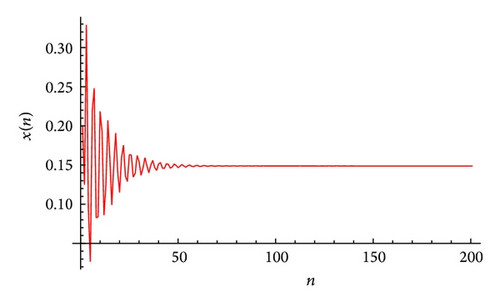
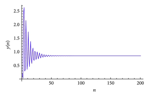
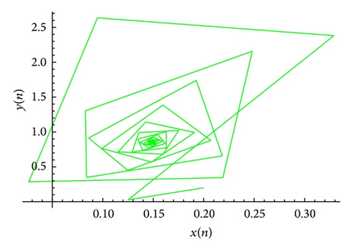
Example 1. Let α = 90, β = 25, γ = 312, α₁ = 2, β₁ = 30, and γ₁ = 5. Then, the system (4) can be written as

()

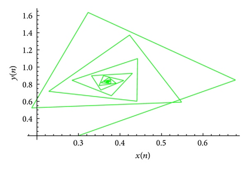
with initial conditions x₋₁ = 11.7, x₀ = 0.2, y₋₁ = 1.8, and y₀ = 0.2.

The plot of x_n for the system (51) is shown in Figure 1, plot of y_n for the system (51) is shown in Figure 2, and its global attractor is shown in Figure 3. The unique positive equilibrium point of the system (51) is given by .

Details are in the caption following the image — **Figure 1**
Open in figure viewer PowerPoint

Plot of x_n for the system (51).

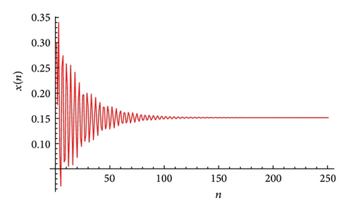
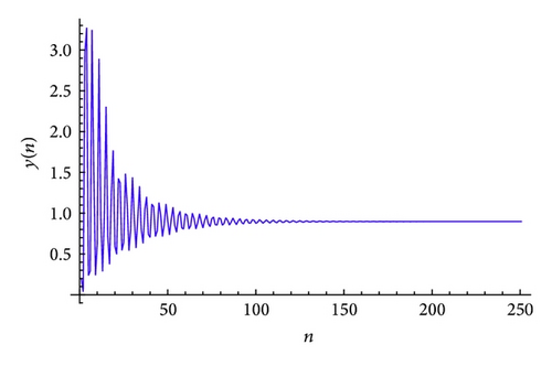
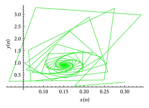
Example 2. Let α = 225, β = 55, γ = 712, α₁ = 1.7, β₁ = 30, and γ₁ = 1.9. Then, the system (4) can be written as

()

with initial conditions x₋₁ = 6.7, x₀ = 0.3, y₋₁ = 1.1, and y₀ = 0.2.

The plot of x_n for the system (52) is shown in Figure 4, plot of y_n for the system (52) is shown in Figure 5, and its global attractor is shown in Figure 6. The unique positive equilibrium point of the system (52) is given by .

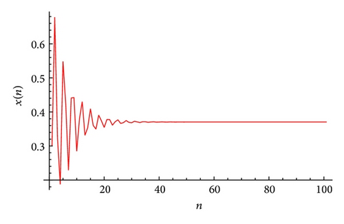
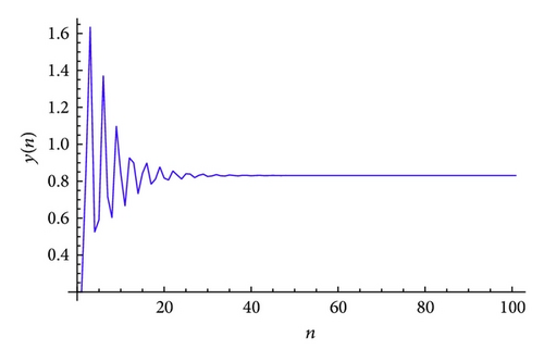
Example 3. Let α = 125, β = 14, γ = 112, α₁ = 15, β₁ = 32, and γ₁ = 0.009. Then, the system (4) can be written as

()

with initial conditions x₋₁ = 0.7, x₀ = 0.3, y₋₁ = 0.9, and y₀ = 0.2.

The plot of x_n for the system (53) is shown in Figure 7, plot of y_n for the system (53) is shown in Figure 8, and its global attractor is shown in Figure 9. The unique positive equilibrium point of the system (53) is given by .

7. Conclusion

This work is related to the qualitative behavior of an exponential system of second-order rational difference equations. We have investigated the existence and uniqueness of positive steady-state of system (4). Under certain parametric conditions the boundedness and persistence of positive solutions are proved. Moreover, we have shown that unique positive equilibrium point of system (4) is locally as well as globally asymptotically stable. The main objective of dynamical systems theory is to predict the global behavior of a system based on the knowledge of its present state. An approach to this problem consists in determining the possible global behaviors of the system and determining which initial conditions lead to these long-term behaviors. Furthermore, rate of convergence of positive solutions of (4) which converge to its unique positive equilibrium point is demonstrated. Finally, some numerical examples are provided to support our theoretical results. These examples are experimental verification of our theoretical discussions.

Conflict of Interests

The authors declare that they have no conflict of interests regarding the publication of this paper.

Acknowledgments

The authors thank the main editor and anonymous referees for their valuable comments and suggestions leading to the improvement of this paper. This work was supported by the Higher Education Commission of Pakistan.

References

1 Zhou Z. and Zou X., Stable periodic solutions in a discrete periodic logistic equation, Applied Mathematics Letters. (2003) 16, no. 2, 165–171, https://doi.org/10.1016/S0893-9659(03)80027-7, MR1962311, 2-s2.0-0037291926.
10.1016/S0893-9659(03)80027-7
CAS Web of Science® Google Scholar
2 Liu X., A note on the existence of periodic solutions in discrete predator-prey models, Applied Mathematical Modelling. Simulation and Computation for Engineering and Environmental Systems. (2010) 34, no. 9, 2477–2483, https://doi.org/10.1016/j.apm.2009.11.012, MR2639527, ZBL1195.39004, 2-s2.0-77952546533.
10.1016/j.apm.2009.11.012
Google Scholar
3 El-Metwally E., Grove E. A., Ladas G., Levins R., and Radin M., On the difference equation , Nonlinear Analysis: Theory, Methods & Applications. (2001) 47, 4623–4634.
10.1016/S0362-546X(01)00575-2
Web of Science® Google Scholar
4 Papaschinopoulos G., Radin M. A., and Schinas C. J., On the system of two difference equations of exponential form: , , Mathematical and Computer Modelling. (2011) 54, 2969–2977.
10.1016/j.mcm.2011.07.019
Google Scholar
5 Papaschinopoulos G. and Schinas C. J., On the dynamics of two exponential type systems of difference equations, Computers & Mathematics with Applications. (2012) 64, no. 7, 2326–2334, https://doi.org/10.1016/j.camwa.2012.04.002, MR2966868, 2-s2.0-84866106469.
10.1016/j.camwa.2012.04.002
Web of Science® Google Scholar
6 Papaschinopoulos G., Radin M., and Schinas C. J., Study of the asymptotic behavior of the solutions of three systems of difference equations of exponential form, Applied Mathematics and Computation. (2012) 218, no. 9, 5310–5318, https://doi.org/10.1016/j.amc.2011.11.014, MR2870051, ZBL1245.39011, 2-s2.0-83555172610.
10.1016/j.amc.2011.11.014
Web of Science® Google Scholar
7 Ozturk I., Bozkurt F., and Ozen S., On the difference equation ), Applied Mathematics and Computation. (2006) 181, no. 2, 1387–1393, https://doi.org/10.1016/j.amc.2006.03.007, MR2270770, 2-s2.0-33750547547.
10.1016/j.amc.2006.03.007
Web of Science® Google Scholar
8 Bozkurt F., Stability analysis of a nonlinear difference equation, International Journal of Modern Nonlinear Theory and Application. (2013) 2, 1–6.
10.4236/ijmnta.2013.21001
Google Scholar
9 Sedaghat H., Nonlinear Difference Equations: Theory with Applications to Social Science Models, 2003, 15, Kluwer Academic Publishers, Dordrecht, The Netherlands, https://doi.org/10.1007/978-94-017-0417-5, MR1967237.
10.1007/978-94-017-0417-5
Google Scholar
10 Kocic V. L. and Ladas G., Global Behavior of Nonlinear Difference Equations of Higher Order with Applications, 1993, Kluwer Academic Publishers, Dordrecht, The Netherlands.
10.1007/978-94-017-1703-8
Google Scholar
11 Grove E. A. and Ladas G., Periodicities in Nonlinear Difference Equations, 2004, Chapman & Hall/CRC, Boca Raton, Fla, USA, MR2193366.
10.1201/9781420037722
Google Scholar
12 Pituk M., More on Poincare′s and PERron′s theorems for difference equations, Journal of Difference Equations and Applications. (2002) 8, no. 3, 201–216, https://doi.org/10.1080/10236190211954, MR1887903, 2-s2.0-0036004717.
10.1080/10236190211954
Web of Science® Google Scholar

Citing Literature

All articles

Behavior of an Exponential System of Difference Equations

Abstract

1. Introduction

2. Boundedness and Persistence

3. Linearized Stability

4. Global Character

5. Rate of Convergence

6. Examples

7. Conclusion

Conflict of Interests

Acknowledgments

References

Citing Literature

Figures

References

Information

About Wiley Online Library

Help & Support

Opportunities

Connect with Wiley

Behavior of an Exponential System of Difference Equations

Abstract

1. Introduction

2. Boundedness and Persistence

3. Linearized Stability

4. Global Character

5. Rate of Convergence

6. Examples

7. Conclusion

Conflict of Interests

Acknowledgments

References

Citing Literature

Figures

References

Related

Information