International Journal of Engineering Mathematics

Volume 2014, Issue 1 485431

Research Article

Open Access

Process Parameter Identification in Thin Film Flows Driven by a Stretching Surface

Satyananda Panda,

Corresponding Author

Satyananda Panda

[email protected]

orcid.org/0000-0003-4219-1725

Department of Mathematics, National Institute of Technology Calicut, Kerala 673601, India nitc.ac.in

Search for more papers by this author

Mathieu Sellier,

Mathieu Sellier

orcid.org/0000-0002-5060-1707

Department of Mechanical Engineering, University of Canterbury, Private Bag 4800, Christchurch 8140, New Zealand canterbury.ac.nz

Search for more papers by this author

M. C. S. Fernando,

M. C. S. Fernando

Department of Mathematics, University of Ruhuna, 81000 Matara, Sri Lanka ruh.ac.lk

Search for more papers by this author

M. K. Abeyratne,

M. K. Abeyratne

Department of Mathematics, University of Ruhuna, 81000 Matara, Sri Lanka ruh.ac.lk

Search for more papers by this author

Satyananda Panda,

Corresponding Author

Satyananda Panda

[email protected]

orcid.org/0000-0003-4219-1725

Department of Mathematics, National Institute of Technology Calicut, Kerala 673601, India nitc.ac.in

Search for more papers by this author

Mathieu Sellier,

Mathieu Sellier

orcid.org/0000-0002-5060-1707

Department of Mechanical Engineering, University of Canterbury, Private Bag 4800, Christchurch 8140, New Zealand canterbury.ac.nz

Search for more papers by this author

M. C. S. Fernando,

M. C. S. Fernando

Department of Mathematics, University of Ruhuna, 81000 Matara, Sri Lanka ruh.ac.lk

Search for more papers by this author

M. K. Abeyratne,

M. K. Abeyratne

Department of Mathematics, University of Ruhuna, 81000 Matara, Sri Lanka ruh.ac.lk

Search for more papers by this author

First published: 21 July 2014

https://doi.org/10.1155/2014/485431

Citations: 2

Academic Editor: Francisco Chinesta

Share a link

Email
Wechat
Bluesky

Abstract

The flow of a thin liquid film over a heated stretching surface is considered in this study. Due to a potential nonuniform temperature distribution on the stretching sheet, a temperature gradient occurs in the fluid which produces surface tension gradient at the free surface of the thin film. As a result, the free surface deforms and these deformations are advected by the flow in the stretching direction. This work focuses on the inverse problem of reconstructing the sheet temperature distribution and the sheet stretch rate from observed free surface variations. This work builds on the analysis of Santra and Dandapat (2009) who, based on the long-wave expansion of the Navier-Stokes equations, formulate a partial differential equation which describes the evolution of the thickness of a film over a nonisothermal stretched surface. In this work, we show that after algebraic manipulation of a discrete form of the governing equations, it is possible to reconstruct either the unknown temperature field on the sheet and hence the resulting heat transfer or the stretching rate of the underlying surface. We illustrate the proposed methodology and test its applicability on a range of test problems.

1. Introduction

The analysis of thin film flow and heat transfer over a stretching surface has been a subject of fundamental importance as it is relevant to several industrial applications such as metal and polymer extrusion, continuous casting, drawing of plastic sheets, or cable coatings to name a few. This industrial context has drawn fluid dynamists and applied mathematicians alike to study this problem from a more canonical angle. The first important contribution to the understanding of this problem is the work of Wang [1] who formulated a mathematical model and developed a solution strategy based on the homotopy analysis method (HAM). The problem has been revisited several times since this seminal work with the inclusion of additional physics or more complex rheology. Andersson et al., for example, extended Wang’s contribution by analyzing the associated heat transfer problem [2, 3], while Noor and Hashim built on the work of Dandapat et al. [4, 5] to consider the thermocapillary and magnetic field effects [6] and Aziz and Hashim that of viscous dissipation [7]. Khan et al. focused on the effect of the temperature-dependency on the viscosity and thermal conductivity on the flow in the film [8] and Andersson et al. extended the standard formulation to power-law fluids [9]. A common feature of the literature cited above is that it is implicitly assumed that the film thickness is uniform in the domain, a required assumption to enable the similarity transformation which reduces the set of partial differential equations to a more tractable one of ordinary differential equations.

Recognizing the restrictions of the plane interface assumption, Dandapat and co-workers were the first to extend the formulation to account for local deformation of the free surface in [10, 11]. The authors exploit the slenderness of the flow domain to derive a long-wave approximation of the Navier-Stokes equations and solve the resulting governing equation using the matched asymptotic method. Lately, this work was extended to include the heat transfer problem [12]. In this work, the nonuniform temperature distribution at the stretching sheet induces an inhomogeneous temperature field in the film. Consequently, a surface temperature gradient develops at the film free surface. As a result of the surface tension gradients, the film thickness varies along the flow and these deformations are advected in the stretching direction.

This work focuses on the flow of a thin liquid film over a heated stretching surface. The aforementioned literature provides solid modeling foundations upon which one can build to indirectly infer process parameters difficult to measure in practice. More specifically, since the developed models correlate the film thickness to the sheet stretch rate and/or temperature through a set of differential equations, it is only natural to wonder whether the knowledge of the film thickness variation allows the reconstruction of either the sheet temperature or the sheet stretch rate. It is precisely this problem which this paper tackles. The motivation for this work is to demonstrate theoretically that it is possible to infer either the stretching rate or the surface temperature from the knowledge of the free surface evolution. This could have interesting practical outcome such as indirectly inferring the heat transfer involved in the process. The solution strategy to solve this inverse problem is inspired from the recent work of Sellier and Panda [13–15], which proposed a strategy to reconstruct an unknown field from free surface data in thin film flows. The general idea is to algebraically manipulate the field equation in order to obtain an explicit differential equation governing the inverse problem. This solution can then be solved using standard numerical techniques. This concept is applied for the first time here to a transient problem. The simplicity of the proposed approach contrasts with the traditional way of dealing with such inverse problems which rely on pde-constrained optimization framework, [16].

The following section briefly describes the mathematical model and numerical solution procedure used to compute the free surface evolution. This section is followed by the development of the inverse problem solution methodology. Some examples illustrating the success of the proposed approach are presented in the penultimate section and finally concluding remarks are drawn in the final section.

2. Description of the Direct Problem

2.1. Mathematical Model

We consider here an unsteady liquid film which lies over a horizontal plane heated elastic sheet as shown in Figure 1. Because surface tension tends to be a monotonically decreasing function of temperature, temperature gradients at the stretching sheet surface induce surface tension variations at the free surface. As regions of high surface tension tend to “pull” on regions of lower surface tension, convective flow cells develop which deform the free surface. This deformation is advected by the flow in the stretching direction. The question this work addresses is how the temperature field at the sheet surface and the stretching velocity can be reconstructed from a known deformation of the free surface.

Details are in the caption following the image — **Figure 1**
Open in figure viewer PowerPoint

Sketch of flow geometry.

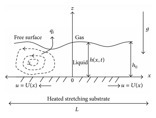
This study is based on the model developed by Santra and Dandapat [12] using the long wave theory. This model is briefly described here for completeness. The elastic sheet lies at z = 0 and the liquid gas interface lies at z = h(x, t), where the x-axis is directed along the stretching sheet and the z-axis is normal to the sheet in the outward direction toward the fluid. Gravity acts along negative z-direction. Further, the surface at z = 0 starts stretching from rest and within a very short time attains the stretching velocity u = U(x). The elastic surface is heated with its temperature Θ a function of x alone and the ambient gas phase is at constant temperature T_a.

The fluid is assumed to be incompressible and Newtonian with constant kinematic viscosity ν, density ρ, specific heat c_p, and thermal conductivity k. The surface tension of the liquid-gas interface decreases linearly with temperature according to

(1)

where T_i is the inter-facial temperature, σ_a is the surface tension at T = T_a, and γ is a positive constant specific to the fluid.

Moreover, Newton’s law of cooling describes the convective heat flux q_i at the interface by

(2)

where T is the temperature in the fluid, n is the unit normal vector on the interface, and α is the rate of heat transfer from the liquid to the ambient gas phase.

Following the analysis of Santra and Dandapat [12] based on the the lubrication equation, the dimensionless evolution equation for film thickness h(x, t) is given by

(3)

where F(h) is the flow discharge given by

(4)

Here the subscript x means partial differentiation with respect to x. The dimensionless numbers are

(i)
the Froude number that expresses the ratio of inertia to body forces;
(ii)
the Prandtl number Pr = ρc_pν/k that represents the ratio of momentum to thermal diffusivity;
(iii)
the Marangoni number that characterizes the relation between the temperature dependent surface tension and viscous forces;
(iv)
the Biot number Bi = αh₀/k that compares the relative magnitudes of resistances to internal conduction and surface convection;
(v)
the dimensionless number S = ϵ²σ_ah₀/ρν² is known as surface tension parameter and ϵ = h₀/L is the aspect ratio.

In the above expressions, h₀ and L are characteristic length scales in the vertical and horizontal directions, respectively. The symbol

stands for the sheet temperature at the origin.

At the origin, we apply the symmetry conditions h_x = 0 and h_xxx = 0 and at the other end of the domain; we assume that the same sheet temperature profiles and the sheet stretching rate continues beyond the computed domain. We also assume that the gradient of the free surface extends out of the computational domain. These boundary conditions are consistent with those mentioned in [12].

2.2. Numerical Solution Procedure

There are many different numerical methods that have been presented in the past for this kind of analysis [12, 17] and in this paper, we mostly follow the finite volume technique described in Sellier and Panda [14] on a uniform grid system with implicit flux discretization.

We discretize our flow domain into the uniform grid and the flow variable h, the steady stretching velocity U, and sheet temperature Θ are located at the cell centers as shown in Figure 2. Let N spatial grid points x₁ < x₂ < ⋯<x_N be equally distributed over the domain [0, L] with spatial increment Δx_i = x_i+1 − x_i = L/(N − 1), i = 1,2, …, N − 1. The numerical solution is sought at the discrete time levels tⁿ, n = 0,1, 2, … with time step Δtⁿ⁺¹ = (tⁿ⁺¹ − tⁿ).

To set up the discrete equation, the function h is approximated over the cell [x_i, x_i+1]. That is the cell average of h over [x_i, x_i+1] is denoted as

(5)

For the given solution

, the solution at the next time level tⁿ⁺¹ is obtained by integrating (3) over the space and time intervals [x_i, x_i+1]×[tⁿ, tⁿ⁺¹]. This yields the following discrete equation:

(6)

for nodes i = 1,2, …, N − 1, where the discrete flux function

is given by

(7)

where face values are evaluated using linear interpolation from nodal values and gradients using forward differences. For example,

(8)

Similar expressions can easily be derived for other terms. The following second-order accurate approximation of the third-order derivative is used:

(9)

The first and the last nodes are located at the boundary and special treatment is required there. Therefore, we apply the boundary conditions in the first node and at the last nodes. In brief, at the first node we have

(10)

where the value of the functions Θ, Θ_x, U, and U_x are known at the cell face x₁. Similarly, we approximate the discrete values at the last node.

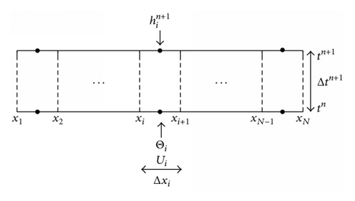
Equation (6) describes an implicit time discretization scheme. Since the governing equation is nonlinear, a system of nonlinear algebraic equations needs to be solved at each time step. We use fsolve in MATLAB for this purpose. A good initial starting guess is required to solve the nonlinear equations. A reasonable initial guess for the free surface is chosen to be unity throughout the discrete domain at the first time step. The solution from the previous time step can be used otherwise. Convergence is usually achieved in less than 10 iterations and the convergence criterion is that the norm of the residuals should be less than 10⁻⁷.

To demonstrate the successful implementation of the proposed finite volume algorithm, the numerical results obtained with the proposed algorithm are compared to those obtained by Santra and Dandapat, [12]. Specifically, the results of Figure 7 in [12] are reproduced here for validation purpose. For this benchmark case, the following temperature distribution and stretching velocity profiles are imposed:

(11)

The temperature profile is illustrated in Figure 3(a). The other nondimensional parameters used in the simulation are reported in the figure caption. The simulation was performed using 150 grid points and time steps of 1.0 (dimensionless units).

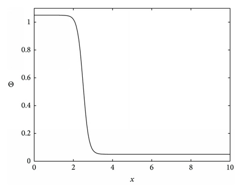
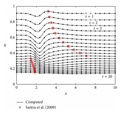
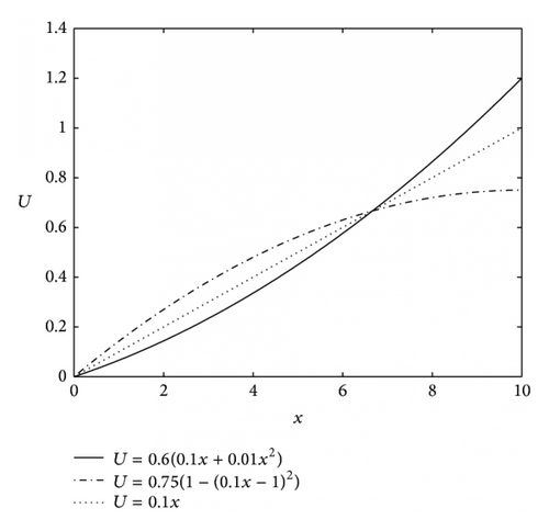
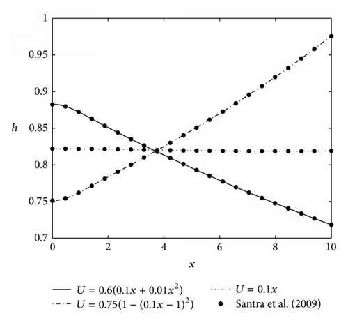
Figure 3(b) illustrates the evolution of free surface at different times. The observed results replicate well those obtained by Santra and Dandapat in [12], and thereby validating the formulation and implementation of the proposed numerical scheme. It is clear from Figure 3(b) that thermocapillary deforms the free surface during the early stages and this deformation is advected downstream by the stretching sheet. To clearly see the motion of the free surface disturbance, the local maximum on each curve is identified with star.

The effect of stretching velocity distribution on film height is demonstrated next. The following Gaussian temperature profile

(12)

is imposed at the sheet and three different stretching velocity distributions are considered:

(13)

The free surface is plotted in Figure 4(b) for the different stretching velocities (illustrated in Figure 4(a)) at a fixed time of t = 2 and the parameters reported in the figure caption. Visual inspection confirms that the computed free surface profiles match well with those computed by Santra and Dandapat in Figure 3 of [12] further demonstrating the accuracy of the proposed numerical approach.

3. The Inverse Problem

The evolution of the free surface provides valuable information on the flow process parameters. Such information can be used to infer unknown conditions otherwise difficult to measure. In the following, we will consider two inverse problems which can be solved using the same conceptual idea.

3.1. Temperature Reconstruction from Two Free Surface Snapshots and Prescribed Stretching Velocity

This first inverse problem consists in inferring the temperature of the stretching sheet from known free surface deformation data and a known stretching velocity distribution over the sheet. The inverse counterpart of the above problem is discussed assuming the transient solution for h exist. More specifically, it is assumed that two free surface profiles at two successive time steps are available. In the following, we reconstruct the sheet temperature distribution Θ from the film thickness profiles obtained by solving the direct problem up to a specific time level t with a prescribed stretching velocity. The main idea behind the reconstruction strategy is that the governing equations, (3) and (4), hold equally well for the forward or the inverse problem. Thus, we can obtain an explicit partial differential equation which “governs” what the temperature distribution needs to be to result in a given film thickness distribution variation. Therefore, unlike traditional inverse problem methods which tend to rely on recasting the reconstruction problem into an optimization one whereby one has to infer the “optimal” temperature distribution which minimizes a given functional, the proposed methodology only involves finding the solution of a partial differential equation. Like the direct problem, we make use of the the same implicit discretized equation (6). Recall the equation as

(14)

This nonlinear discrete equation could equally be written as

(15)

where the bold font indicates the vector of discrete values. The explicit form of the operator

is lengthy and not reported here. With the governing equation in this form, it becomes apparent that this equation describes three possible problems. The usual forward problem, as it is usually described, is recovered if we assume that hⁿ, Θ, and U are known and hⁿ⁺¹ is sought. The two inverse problems of interest here are recovered if

(i)
hⁿ⁺¹, hⁿ, and U are known and Θ is sought;
(ii)
hⁿ⁺¹, hⁿ, and Θ are known and U is sought;

Irrespective of the inverse problem considered, (15) is an implicit equation for the temperature distribution (given the stretching rate), or the stretching rate (given the temperature distribution). Boundary conditions similar to the ones used for the forward problem are implemented in the inverse problem. Equation (15) is solved implicitly in the scientific computing program MATLAB using the fsolve routine for the reconstruction of Θ from the knowledge of the film thickness distribution at two successive time steps and the temperature at the end points of the flow domain. An initial guess of zero temperature distribution, that is, Θ(x) = 0, is considered for the implicit solver.

For the first test case, the artificial “experimental” free surface data is obtained for the prescribed linear stretching velocity U(x) = x and the following sine temperature profile:

(16)

Additional noise with a standard uniform distribution is added to the obtained film thickness profile to replicate the likely measurement uncertainty. The amplitude of the added noise was either 3% of the total film thickness variation or 5%. Without any prior processing of the noisy data, the reconstruction algorithm invariably failed. However, the algorithm was successful if a cubic spline was first fitted through the noisy film thickness variation. The MATLAB function csaps() was used for this purpose with a smoothing parameter set to 0.9, [18]. The nondimensional parameters used in the simulation are reported in the figure caption. The number of grid points is 150 and time steps of 0.03 are used in the simulation. The corresponding free surface profile with and without noise at t = 0.3 is shown in Figure 5(a). Figure 5(b) shows the reconstructed and the actual temperature profiles. Without noise, these two profiles are indistinguishable thereby validating the conceptual reconstruction idea and the implementation of the algorithm. Given the smoothness of the actual temperature profile, it comes as little surprise that even with the addition of 3% or 5% noise on the free surface data, the reconstructed temperature profile still is in good agreement with the actual one. This highlights the robustness of the proposed methodology even in the presence of noise.

The ability of the proposed algorithm to reconstruct temperature profiles with a much steeper variation is tested in the next test case. The artificial temperature profile given by a smoothed step temperature function, that is,

(17)

As in the previous case, 3% and 5% noise was then added to the film thickness profiles. Cubic splines were then fitted through these free surface profiles and used as input to the reconstruction algorithm. The resulting free surface profiles with and without noise at t = 20 can be seen in Figure 6(a). It is apparent from these profiles that the film thickness variations occur on a much shorter length scale which will lead to a more difficult test case for the reconstruction algorithm, as one would expect. Reconstruction results can be seen on Figure 6(b) without noise, for 2% added noise, and for 5% added noise. Without noise, it is apparent that the actual and reconstructed temperature profiles are strictly identical again confirming that it is possible to reconstruct the surface temperature from the knowledge of two successive free surface profiles and the stretching velocity. It is also clear that the actual and reconstructed temperature profiles are still in reasonable agreement when noise is added to the input data. The reconstruction algorithm only mildly amplifies the input noise. The quality of the reconstruction for this second case is not as good as for the first one and one can attribute this to the difficulty of fitting a good representative cubic spline through rapidly varying data. Hence, one would expect this reconstruction algorithm to work best when the unknown temperature profile does not vary too rapidly.

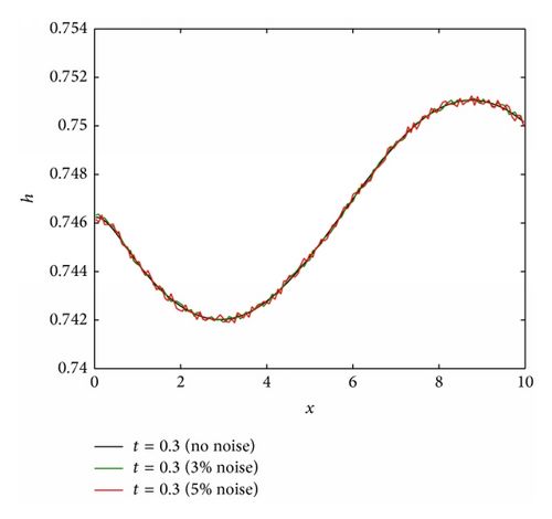
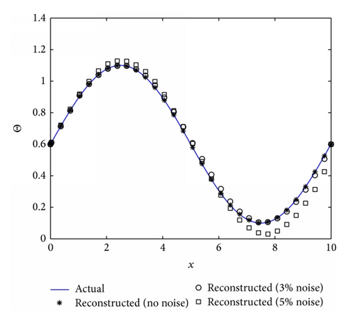
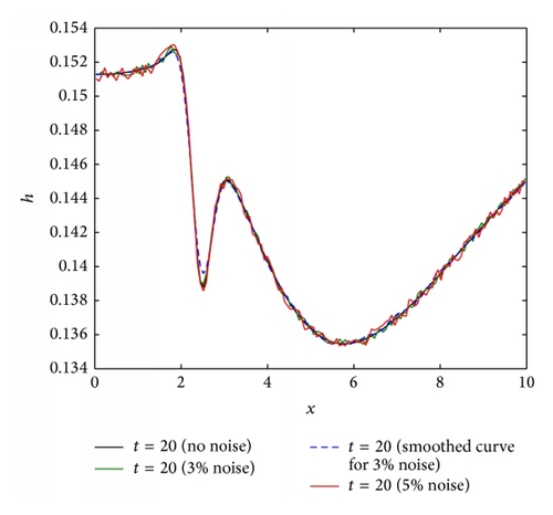
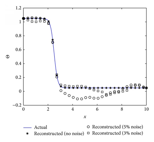
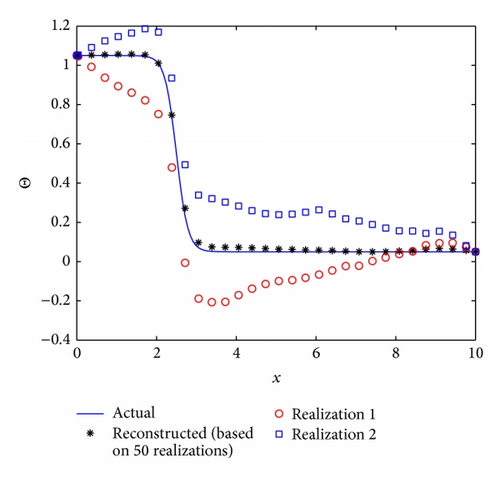
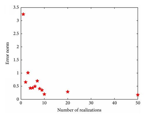
In the inevitable presence of noise in an experimental system, the natural procedure is to run several realizations of the same experiment and average the output data. This is precisely what we proceeded to do in order to check whether, as the number of realization increases, the agreement between the reconstructed and actual temperature profile improves, as one would expect. Results are reported in Figure 7 for the 5% noise case for which the agreement between the actual and reconstructed temperature profiles was the poorest. In effect, we ran numerous reconstruction with 5% noise added to the film thickness and averaged the reconstructed temperature profiles. Figure 7(a) shows two realizations of the reconstructed temperature profiles (Realizations 1 and 2) which are rather poor. However, averaging the reconstructed temperature profile over 50 realizations yields a very good agreement with the actual distribution, as anticipated. Figure 7(b) shows the norm of the difference between the actual and reconstructed temperature profiles. It is clear from this graph that the norm decreases very rapidly for the first few realizations with very marginal reduction of this norm between 10 to 50 realizations. This indicates that, in practice, few realizations of the experiment would be necessary in order to obtain a reliable reconstruction of the temperature distribution.

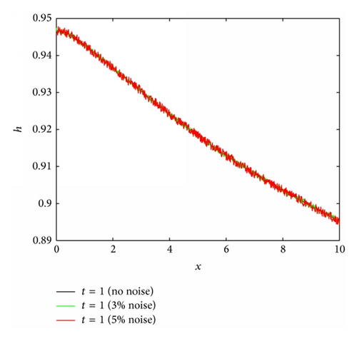
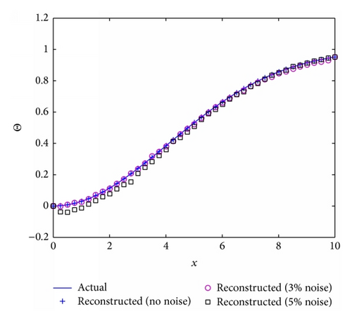
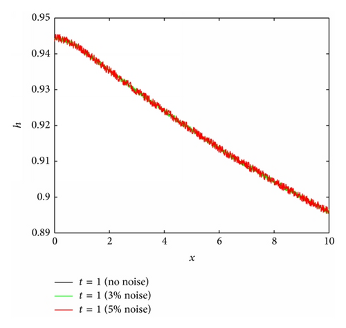
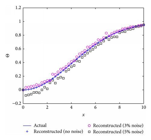
To explore the effects of the Prandtl number (Pr), the Biot number (Bi), and the surface tension parameter (S) on the reconstruction algorithm the algorithm was run for four different scenarios where Fr = 1, M = 4, and ϵ = 0.05 are fixed and the Biot number, Prandtl number and surface tension parameter vary, that is, Bi ∈ {0.1,1, 2}, Pr ∈ {1,5}, and S ∈ {1,2}. A nonlinear parabolic (concave) profile is considered for the stretching velocity that is, U = 0.6(0.1x + 0.005x²) for all four cases. Considering Figures 8(b), 9(b), and 10(b), it can be seen that the reconstruction algorithm recovers the temperature profile extremely well without noise even if the imposed stretching velocity is nonlinear. For 2% and 5% added noise, the quality of the reconstruction is still reasonable. The corresponding free surface profiles can be seen in Figures 8(a), 9(a), and 10(a). Slightly larger discrepancies can be observed when the surface tension parameter is increased from S = 1 to S = 2, see Figure 11(b).

3.2. Stretching Velocity Reconstruction from Two Free Surface Snapshots and Prescribed Temperature Distribution

It is clear from the work of [10–12] that the stretching velocity plays an important role in the evolution of the thin film height. In addition to the Marangoni effect, the type of stretching applied at the bottom sheet mainly influences the film profile. In the following analysis, we discuss how to reconstruct the stretching velocity from given free surface data and temperature distribution at the surface. For this purpose, we first solve the forward problem for the film thickness profile up to a particular time for a given temperature distribution and stretching sheet velocity. To reconstruct the stretching velocity profile, we consider the same governing equations: (3) in continuous form and (6) in discretized form. In order to solve the nonlinear algebraic equation (6) for the stretching velocity U from the known two successive free surface profiles and the temperature function Θ, we first prescribe the stretching sheet velocity at the boundary points and then solve the equation using MATLAB fsolve routine. It is observed that for any nonzero constant initial guess, the MATLAB solver converges within less than 10 iterations.

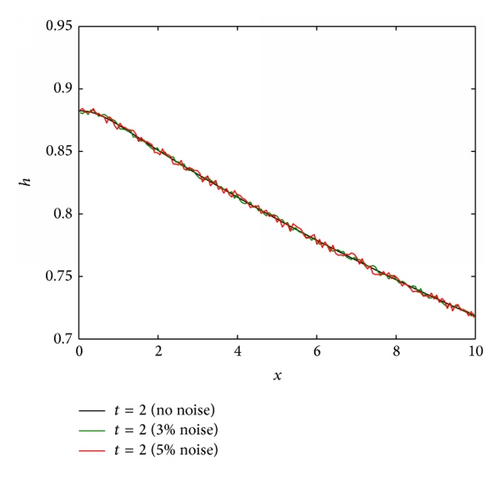
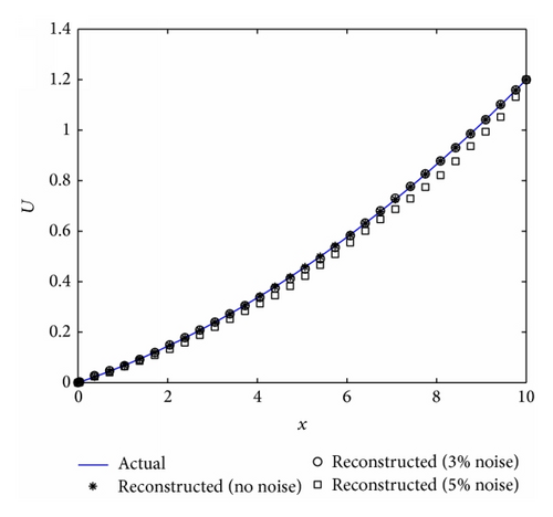
For the first case, the film thickness is obtained up to a particular time of t = 2 for the stretching velocity U(x) = 0.6(0.1x + 0.01x²), and temperature profile is given by (12). The other flow parameters used in the simulation are reported in the figure caption. The transient solution is obtained by solving (6), for 150 grid points and time steps of 0.1. The film thickness at t = 2 is shown in Figure 12(a) without noise and with 3% and 5% noise. Figure 12(b) shows the reconstructed and actual stretching velocity profiles. In the absence of noise, the perfect agreement between the two profiles confirms that the reconstruction algorithm is able to recover the stretching velocity equally well as it could recover the substrate temperature profile. The addition of up to 5% noise still lead to a reasonable reconstruction.

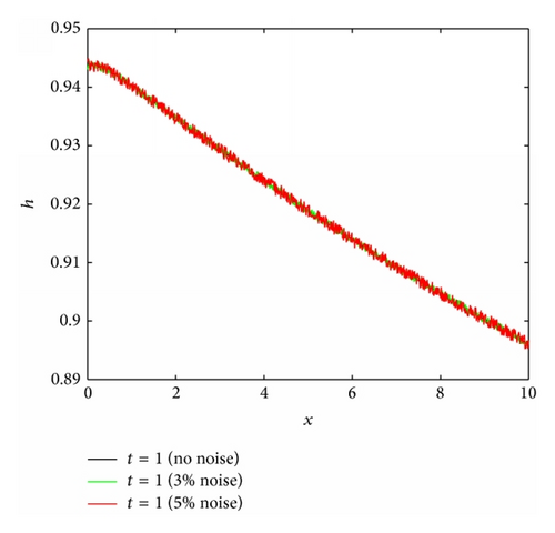
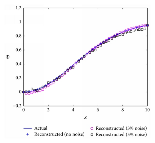
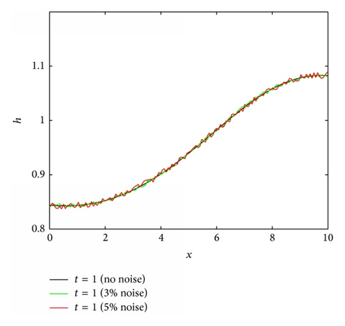
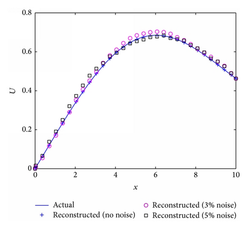
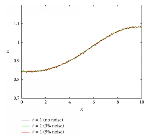
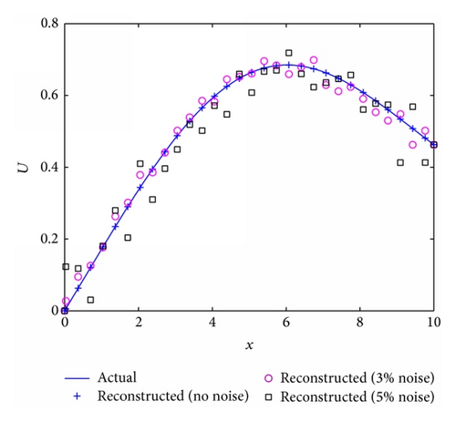
For the second case, the film thickness is obtained up to a particular time of t = 1 for the nonmonotonic stretching velocity and temperature profile . The other flow parameters used in the simulation are reported in the figure caption. The simulation results for reconstructed surface velocity without surface tension (S = 0) and with surface tension (S = 0.1) are given in Figures 13(b) and 14(b), respectively. In the absence of surface tension the reconstruction algorithm is able to recover the stretching velocity profile. It can be seen that with the inclusion of surface tension the algorithm perfectly reconstruct the sheet velocity in the absence of noise (Figure 14(b)). With the addition of noise the reconstructed results differ mildly from the actual one.

4. Concluding Remarks

A solution strategy is presented in this work to reconstruct the surface temperature profile or the surface stretching rate from the knowledge of the thickness at a given time and its rate of change. The main idea is simply based on a rearrangement of the equations derived by Santra and Dandapat in [12] for nonisothermal thin liquid films on stretching surfaces. This rearrangement of the governing equations leads to an explicit partial differential equation which governs the inverse problem. This allows to solve the inverse problem in “one shot” which is a considerable advantage compared to the traditional way of approaching such inverse problems based on pde-constrained optimization theory. We have demonstrated that the algorithm is quite robust in the sense that noise in the input data is not too amplified provided the input data is smoothed using a cubic spline. Whilst the focus of this paper is on the presentation of the conceptual idea, future work will assess the feasibility and practicality of the suggested approach using true experimental data.

Conflict of Interests

The authors declare that there is no conflict of interests regarding the publication of this paper.

References

1 Wang B., Liquid film on an unsteady stretching surface, Quarterly of Applied Mathematics. (1990) 48, no. 4, 601–610, MR1079908.
Google Scholar
2 Andersson H. I., Aarseth J. B., and Dandapat B. S., Heat transfer in a liquid film on an unsteady stretching surface, International Journal of Heat and Mass Transfer. (2000) 43, no. 1, 69–74, https://doi.org/10.1016/S0017-9310(99)00123-4, ZBLl1042.76507, 2-s2.0-0342632546.
10.1016/S0017-9310(99)00123-4
Google Scholar
3 Liu I.-C. and Andersson H. I., Heat transfer in a liquid film on an unsteady stretching sheet, International Journal of Thermal Sciences. (2008) 47, no. 6, 766–772, https://doi.org/10.1016/j.ijthermalsci.2007.06.001, 2-s2.0-40749114657.
Google Scholar
4 Dandapat B. S., Santra B., and Andersson H. I., Thermocapillarity in a liquid film on an unsteady stretching surface, International Journal of Heat and Mass Transfer. (2003) 46, no. 16, 3009–3015, https://doi.org/10.1016/S0017-9310(03)00078-4, ZBLl1048.76502, 2-s2.0-0037870117.
10.1016/S0017-9310(03)00078-4
Google Scholar
5 Dandapat B. S., Santra B., and Vajravelu K., The effects of variable fluid properties and thermocapillarity on the flow of a thin film on an unsteady stretching sheet, International Journal of Heat and Mass Transfer. (2007) 50, no. 5-6, 991–996, https://doi.org/10.1016/j.ijheatmasstransfer.2006.08.007, ZBLl1124.80317, 2-s2.0-33846570463.
Google Scholar
6 Noor N. F. M. and Hashim I., Thermocapillarity and magnetic field effects in a thin liquid film on an unsteady stretching surface, International Journal of Heat and Mass Transfer. (2010) 53, no. 9-10, 2044–2051, https://doi.org/10.1016/j.ijheatmasstransfer.2009.12.052, ZBLl1190.80025, 2-s2.0-76749168046.
Google Scholar
7 Aziz R. C. and Hashim I., Liquid film on unsteady stretching sheet with general surface temperature and viscous dissipation, Chinese Physics Letters. (2010) 27, no. 11, 110202, https://doi.org/10.1088/0256-307X/27/11/110202, 2-s2.0-78649342141.
Google Scholar
8 Khan Y., Wu Q., Faraz N., and Yildirim A., The effects of variable viscosity and thermal conductivity on a thin film flow over a shrinking/stretching sheet, Computers & Mathematics with Applications. (2011) 61, no. 11, 3391–3399, https://doi.org/10.1016/j.camwa.2011.04.053, MR2802005, 2-s2.0-79956344151.
Google Scholar
9 Andersson H. I., Aarseth J. B., Braud N., and Dandapat B. S., Flow of a power-law fluid film on an unsteady stretching surface, Journal of Non-Newtonian Fluid Mechanics. (1996) 62, no. 1, 1–8, https://doi.org/10.1016/0377-0257(95)01392-X, 2-s2.0-0029656469.
10.1016/0377-0257(95)01392-X
Google Scholar
10 Dandapat B. S., Kitamura A., and Santra B., Transient film profile of thin liquid film flow on a stretching surface, Zeitschrift für angewandte Mathematik und Physik ZAMP. (2006) 57, no. 4, 623–635, https://doi.org/10.1007/s00033-005-0040-7, MR2244810, 2-s2.0-33745924700.
Google Scholar
11 Dandapat B. S. and Maity S., Flow of a thin liquid film on an unsteady stretching sheet, Physics of Fluids. (2006) 18, no. 10, 7, 102101, https://doi.org/10.1063/1.2360256, MR2291682, 2-s2.0-33750592086.
Google Scholar
12 Santra B. and Dandapat B. S., Unsteady thin-film flow over a heated stretching sheet, International Journal of Heat and Mass Transfer. (2009) 52, 1965–1970, https://doi.org/10.1016/j.ijheatmasstransfer.2008.09.036.
Google Scholar
13 Sellier M., Substrate design or reconstruction from free surface data for thin film flows, Physics of Fluids. (2008) 20, no. 6, 062106, https://doi.org/10.1063/1.2939404, ZBLl1182.76678, 2-s2.0-47149094057.
Web of Science® Google Scholar
14 Sellier M. and Panda S., Surface temperature reconstruction based on the thermocapillary effect, The ANZIAM Journal. (2010) 52, no. 2, 146–159, https://doi.org/10.1017/S1446181111000654, MR2832609, 2-s2.0-82555175812.
Google Scholar
15 Sellier M. and Panda S., Inverse temperature reconstruction in thermocapillary-driven thin liquid films, International Journal of Numerical Analysis and Modeling B. (2012) 3, no. 3, 285–296, MR3000183.
Google Scholar
16 Pironneau O., Optimal Shape Design for Elliptic Systems, 1984, Springer, New York, NY, USA, https://doi.org/10.1007/978-3-642-87722-3, MR725856.
Google Scholar
17 Ha Y., Kim Y.-J., and Myers T. G., On the numerical solution of a driven thin film equation, Journal of Computational Physics. (2008) 227, no. 15, 7246–7263, https://doi.org/10.1016/j.jcp.2008.04.007, MR2433970, 2-s2.0-45449092536.
Google Scholar
18 The MathWorks Inc., MATLAB R2011b Documentation, 2011, The MathWorks Inc..
Google Scholar

Citing Literature

All articles

Process Parameter Identification in Thin Film Flows Driven by a Stretching Surface

Abstract

1. Introduction

2. Description of the Direct Problem

2.1. Mathematical Model

2.2. Numerical Solution Procedure

3. The Inverse Problem

3.1. Temperature Reconstruction from Two Free Surface Snapshots and Prescribed Stretching Velocity

3.2. Stretching Velocity Reconstruction from Two Free Surface Snapshots and Prescribed Temperature Distribution

4. Concluding Remarks

Conflict of Interests

References

Citing Literature

Figures

References

Information

About Wiley Online Library

Help & Support

Opportunities

Connect with Wiley

Process Parameter Identification in Thin Film Flows Driven by a Stretching Surface

Abstract

1. Introduction

2. Description of the Direct Problem

2.1. Mathematical Model

2.2. Numerical Solution Procedure

3. The Inverse Problem

3.1. Temperature Reconstruction from Two Free Surface Snapshots and Prescribed Stretching Velocity

3.2. Stretching Velocity Reconstruction from Two Free Surface Snapshots and Prescribed Temperature Distribution

4. Concluding Remarks

Conflict of Interests

References

Citing Literature

Figures

References

Related

Information