Dynamics Analysis of a Class of Delayed Economic Model
Abstract
This investigation aims at developing a methodology to establish stability and bifurcation dynamics generated by a class of delayed economic model, whose state variable is described by the scalar delay differential equation of the form d2p(t)/dt2 = −μδ(p(t))(dp(t)/dt) − μbp(t − τ1) −μ(a0p(t − τ2)/(a1 + p(t − τ2))) + μ(d0 − g0). At appropriate parameter values, linear stability and Hopf bifurcation including its direction and stability of the economic model are obtained. The main tools to obtain our results are the normal form method and the center manifold theory introduced by Hassard. Simulations show that the theoretically predicted values are in excellent agreement with the numerically observed behavior. Our results extend and complement some earlier publications.
1. Introduction
Trade cycles, business cycles, and fluctuations in the price and supply of various commodities have attracted the attention of economists for well over one hundred years and possible more than thousands of years [1]. In the case of the most models discussed earlier in the literature, it is assumed that each economic agent has instantaneous information about its own as well as its rivals′ behavior. Many authors often attributed these fluctuations to instantaneous information factors. This assumption is mathematically convenient but does not fully describe real economic situations in which there are always time delays between the times when information is obtained and the times when the decisions are implemented. In recent years it has been recognized in continuous-time economic dynamics that a delay differential equation is useful to describe the periodic and aperiodic behavior of economic variables [2–7]. Time delays usually cause the models to generate not only periodic cycles but also chaotic behavior for certain values of the shape parameter of the production function. With the infinite dimensionality created by a fixed-time delay, even a single first-order equation is transformed into an equation with a sufficient number of degrees of freedom to permit the occurrence of complex dynamics involving chaotic phenomena. This finding indicates that fixed-time delay models of a dynamic economy may explain various complex dynamic behaviors of the economic variables. For decades, a lot of effort has been devoted to deepen the understanding of economic complexity including chaotic behavior, stability, and basins of attractions. In [2], Matsumoto and Szidarovszky and in [3], Akio and Ferenc investigate a continuous-time neoclassical growth model with time delay and study the dynamics of the delayed model. In [4], Bélair and Mackey develop a model of price adjustment with production delays. In [5], Zhang et al. consider a differential-algebraic biological economic system with time delay and harvesting where the dynamics is logistic with carrying capacity proportional to prey population. Howroyd and Russel detect the stability conditions of delay output adjustment processes in a general N-firm oligopoly with fixed time delays [6]. Matsumoto and Szidarovszky introduce a fixed delay in production and a mound-shaped production function into the neoclassical one-sector growth model and show the birth of complex dynamics [2]. Considering about a delay in the production process, Li establish the single commodity price-inventory control model [7].
It is well known that persistent oscillations are one of the most ubiquitous forms by which economic phenomena may be observed [8]. Limit cycles are the simplest nonlinear phenomena, for example, they are the simplest example of how the interaction between economic forces may compel a system to abandon its steady state and start to steadily oscillate. Just as reported by Manfredi and Fanti [9], the detection of stable oscillations, for example, stable limit cycles, in continuous-time systems, is intimately related with the notion of Hopf bifurcation. Hopf bifurcation is important in economics. There are at least three reasons. First, it is always the outcome of a fully endogenous interaction between (nonlinear) economic forces. Second, it is a local bifurcation, thus much in spirit with the common belief of our science by which economic systems are generally close to their equilibrium state. Third, because it implieslocal oscillations, which are the normal route through which disequilibrium manifests itself when the equilibrating forces operating in the economy are relaxed (e.g., the adjustment process of a Walrasian market). For instance, when oscillations persist in a market normally in equilibrium (in the absence of stochastic and seasonal perturbations), it is very likely that these oscillations are the outcome of a Hopf bifurcation. So it is necessary for us to research the Hopf bifurcation in the economic system.
In the case of the most models discussed in the mentioned literature, only one delay appears in the models. Considering that the consumer memory plays an important role in the process of economic activities, just as pointed out by Li [7], bringing another delay might be better candidates for some purposes and would be of great interest. In this paper, we will generalize an economic model with the help of bringing two delays. In specifying how consumer behavior affects commodity demand, we will assume that the behavior is influenced not only by the instantaneous price, but also by the information regarding past prices. As the fact that the quantity supplied may not increase infinitely during the price increasing, similar to [7], we also assume the supply function to be fractional linear function. This investigation aims at developing a methodology to establish stability and bifurcation dynamics generated by the new delayed economic model.
The organization of the rest of this paper is as follows. In Section 2, we establish an economic model with two delays combing with the model considered in [7]. In Section 3, we take the delays as the parameters and use the distribution theory of the transcendental equation root [10] and the theory of Hopf bifurcation about functional differential equation [11] to discuss the stability of the equilibrium point for economic system and the existence of Hopf bifurcation. In Section 4, we apply the normal form theory and center manifold theory to investigate the bifurcation direction and the stability of periodic solution. In Section 5, an example with numerical simulations is arranged to illustrate the obtained results.
2. Characterization of a Generalized Delayed Economic Model
Considering a single commodity market, the quantity of supplied and demanded can be regarded as the function of time, namely, G(t) and D(t). The inventory and the level of inventory are recorded, respectively, as S(t) and .
- (H1)
The inequality hold: d0 > g0.
- (H2)
The inequality hold: δ(p*) > 0, where p* is a positive equilibrium point.
- (H3)
The inequality hold: b < a0a1/(a1 + p*) 2, where p* is a positive equilibrium point.
3. Stability Analysis and the Existence of Hopf Bifurcation
At first, we will show that system (8) has only one positive equilibrium point under some assumption. We state the following theorem.
Theorem 1. If the inequality (H1) holds: d0 > g0, then system (8) has only one positive equilibrium point.
Proof. Without loss of generality, we may assume that
Assume p* to be the equilibrium point of system (8), one can show that (p*, 0) is the equilibrium point of system (11). Therefore, one can obtain
It is well known that the equilibrium (0,0) is asymptotically stable if all roots of the characteristic equation (17) have negative real parts. Now we reach the position to study the distribution of the roots of (17). We will consider three cases as follows: (Case 1): τ1 = 0, τ2 = 0; (Case 2): τ1 = 0, τ2 > 0; and (Case 3): τ2 > τ1 > 0.
Case 1. τ1 = 0, τ2 = 0.
Proposition 2. If τ1 = 0, τ2 = 0 and the inequality (H2) hold: δ(p*) > 0, then the equilibrium point (0,0) of system (15) is asymptotically stable.
Proof. As the inequality (H2) holds, then the characteristic equation (17) turns to be
Case 2 (τ1 = 0, τ2 > 0). If τ1 = 0, τ2 > 0, then the characteristic equation (17) takes the following form:
Lemma 3. If the inequality (H3) holds: b < a0a1/(a1 + p*) 2, and τ2 = τ2n, then E(λ) = 0 has the only pair of purely imaginary roots λ = ±iω, where
Proof. If λ = iω(τ2) (ω(τ2) > 0) is a root of (19), then
Denote λ(τ2) = α(τ2) + iω(τ2); then the root of (19) satisfies: α(τ2n) = 0, ω(τ2n) = ω.
Lemma 4. If one chooses
Proof. Taking the derivative of E(λ) = 0 with respect to τ2, we get
Based on the lemmas presented previous and the classical Hopf-Bifurcation-Theorem (see, [11, pages 245–249]), we have the following result.
Theorem 5. Assume that the inequalities (H1)–(H3) hold, then one has the following result.
- (1)
If τ2 ∈ [0, τ20), all roots of (19) have negative real parts. Namely, the equilibrium (0,0) of system (15) is locally asymptotically stable.
- (2)
If τ2 = τ20, (19) have a pair of purely imaginary roots ±iω, all the other roots have negative real parts. That is to say, system (15) undergoes a Hopf bifurcation at τ2 = τ20.
- (3)
If τ2 > τ20, (19) has roots of positive real parts. Namely the equilibrium (0,0) of system (15) is unstable.
Case 3 (τ2 > τ1 > 0). We now discuss the stability of equilibrium (0,0) when τ1 > 0, τ2 = τ ∈ [0, τ20).
Let λ = iω(τ1)(ω(τ1) > 0) be the root of (17) and substitute it into (17), we have
If (34) has no root or negative root, all the roots of (17) have negative real part. If it has positive roots, we know that the number of positive roots is finite. Denote them to be ωi (i = 1,2, 3 … , N). From (33), we can get
Theorem 6. Assume that the inequalities (H1)–(H3) hold, then one has the following result.
4. Direction and Stability of the Bifurcation
In this section, formula for determining the direction of Hopf bifurcation and the stability of bifurcation periodic solution of system (11) at , τ2 = τ ∈ [0, τ20) will be presented by employing the normal form method and center manifold theorem introduced by Hassard et al. in [12]. More precisely, we will compute the reduced system on the center manifold with the pair of conjugate complex, purely imaginary solution of the characteristic equation (17). By this reduction, we can determine the Hopf bifurcation direction, that is, to answer the question of whether the bifurcation branch of periodic solution exists locally for supercritical bifurcation or subcritical bifurcation.
As Lk is a one-parameter family of bounded linear operator in C[−τ*, 0], by the Rise Representation Theorem, there exists a matrix whose components are bounded variation functions η(θ, k), θ ∈ [−τ*, 0] such that , Φ ∈ C[−τ*, 0]. Actually, we can take η(θ, k) = A1(k)δ(θ) +A2(k)δ(θ + 1) + A3(k)δ(θ + τ*), where δ is Dirac delta function.
Denote A(0) = A, R(0) = R, Ai(0) = Ai (i = 1,2, 3), η(θ, 0) = η(θ).
We easily obtain that ±iτ0ω0 are eigenvalues of (17) by the translation t → t/τ1. Then we have the following lemma.
Lemma 7. is the eigenvector corresponding to iτ0ω0 and is the eigenvector of A* corresponding to −iτ0ω0. 〈q*(s), q(θ)〉 = 1, , where
Proof. Letting q(θ) be the eigenvector of corresponding to iτ0ω0, we have
From (43), we can obtain
Letting be the eigenvector of A* corresponding to −iτ0ω0, based on (48), (50), we have
Now we compute 〈q*(s), q(θ)〉 as the following:
In the remainder of this section, we use the same notation as in [12]. We first compute the center manifold C0 at k = 0.
Theorem 8. Using (81), one can compute the values of C1(0), μ2, β2, T2. Therefore, we can answer the question of whether the bifurcation branch of periodic solution exists locally for supercritical bifurcation or subcritical bifurcation as the following.
- (i)
μ2 determines the directions of the Hopf bifurcation: if μ2 > 0 (μ2 < 0), then the Hopf bifurcation is supercritical (subcritical) and the bifurcating periodic solutions exists for k = 0.
- (ii)
β2 determines the stability of the bifurcating periodic solutions: the bifurcating periodic solutions are stable (unstable) if β2 < 0 (β2 > 0).
- (iii)
T2 determines the period of the bifurcating periodic solutions: the period increases (decreases), if T2 > 0 (T2 < 0).
5. Numerical Simulation Example
Example 9. Consider a single commodity market model as follows:
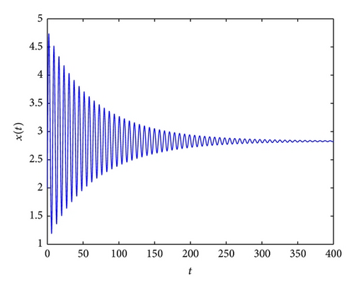
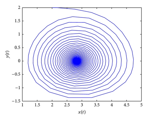
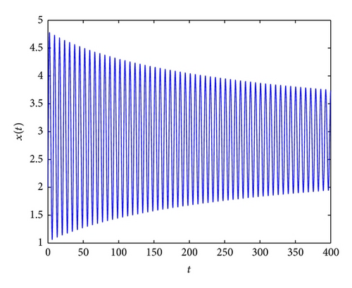
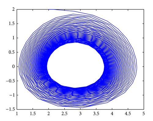
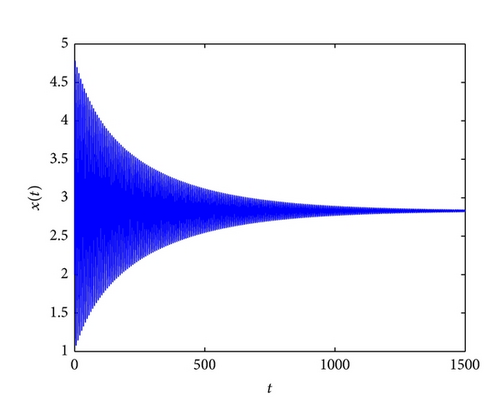
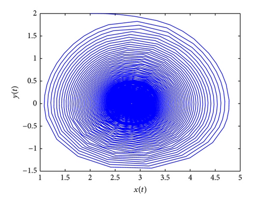
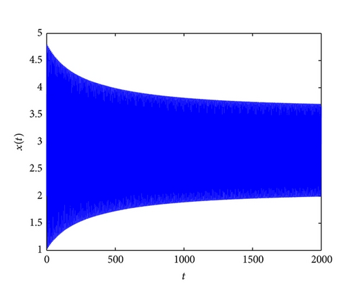
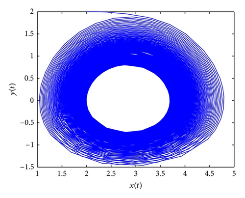
If one choose τ1 = 0, τ2 > 0, from Lemma 3, we can calculate that ω = 0.8875, τ20 = 0.7237, and τ20 is the the critical value for Hopf bifurcation. It follows from Theorem 5 that if τ2 ∈ (0,0.7237), (p*, 0) is asymptotically stable. System (82) undergoes a Hopf bifurcation at τ2 = 0.7237. These conclusions are verified by the numerical simulation in Figures 1, 2, 3, and 4.
When τ2 > τ1 > 0, we can choose τ2 = τ = 0.68; from (34) and (35), we can calculate that ω0 = 0.9203, ; from (37), we have . It follows from Theorem 6 that (p*, 0) is asymptotically stable as far as and system (82) undergoes a Hopf bifurcation when . Furthermore, using Lemma 7, after simple computation, we have
6. Conclusion
The delay in production process has been considered in many economic models. However, few of them considered the delay of consumer consumption. In this paper, we first establish a class of economic models with two delays; the delay in production process and consumer consumption are both considered, and then the dynamics of this system have been investigated. Specifically, stability of equilibrium point and the existence of Hopf bifurcation, in great detail, are studied. We have derived some sufficient conditions to ensure that all the characteristic roots have negative real parts. We also show that a Hopf Bifurcation will occur once some parameters pass through critical values; that is, a family of periodic orbits bifurcates from the positive equilibrium point. At last, the direction of Hopf bifurcation and the stability of the bifurcating periodic orbits are discussed by applying the normal form theory and the center manifold theorem. Simulations show that the theoretically predicted values are in excellent agreement with the numerically observed behavior. Our results extend and complement some earlier publications.
Acknowledgments
The authors are extremely grateful to the editor and the anonymous reviewers for their constructive and valuable comments, which have contributed much to the improvement of this paper. This work was jointly supported by the National Natural Science Foundation of China under Grants nos. 11101053, 70921001, and 71171024, the Key Project of Chinese Ministry of Education under Grant no. 211118, the Excellent Youth Foundation of Educational Committee of Hunan Provincial no. 10B002, and the Scientific Research Funds of Hunan Provincial Science and Technology Department of China.


