Volume 2013, Issue 1 795682

Research Article

Open Access

A New Class of the Planar Networks with High Clustering and High Entropy

Guona Hu,

Guona Hu

Department of Mathematics, Qinghai Normal University, Xining, Qinghai 810008, China qhnu.edu.cn

Search for more papers by this author

Yuzhi Xiao,

Yuzhi Xiao

School of Computer Science, Shaanxi Normal University, Xi′an, Shaanxi 710062, China snnu.edu.cn

Department of Computer Science, Qinghai Normal University, Xining, Qinghai 810008, China qhnu.edu.cn

Search for more papers by this author

Huanshen Jia,

Huanshen Jia

Department of Mathematics, Qinghai Normal University, Xining, Qinghai 810008, China qhnu.edu.cn

Search for more papers by this author

Haixing Zhao,

Corresponding Author

Haixing Zhao

[email protected]

School of Computer Science, Shaanxi Normal University, Xi′an, Shaanxi 710062, China snnu.edu.cn

Department of Computer Science, Qinghai Normal University, Xining, Qinghai 810008, China qhnu.edu.cn

Search for more papers by this author

Guona Hu,

Guona Hu

Department of Mathematics, Qinghai Normal University, Xining, Qinghai 810008, China qhnu.edu.cn

Search for more papers by this author

Yuzhi Xiao,

Yuzhi Xiao

School of Computer Science, Shaanxi Normal University, Xi′an, Shaanxi 710062, China snnu.edu.cn

Department of Computer Science, Qinghai Normal University, Xining, Qinghai 810008, China qhnu.edu.cn

Search for more papers by this author

Huanshen Jia,

Huanshen Jia

Department of Mathematics, Qinghai Normal University, Xining, Qinghai 810008, China qhnu.edu.cn

Search for more papers by this author

Haixing Zhao,

Corresponding Author

Haixing Zhao

[email protected]

School of Computer Science, Shaanxi Normal University, Xi′an, Shaanxi 710062, China snnu.edu.cn

Department of Computer Science, Qinghai Normal University, Xining, Qinghai 810008, China qhnu.edu.cn

Search for more papers by this author

First published: 07 December 2013

https://doi.org/10.1155/2013/795682

Citations: 3

Academic Editor: Jinde Cao

Share a link

Email
Wechat
Bluesky

Abstract

Small-world networks are ubiquitous in real-life systems, such as the World Wide Web, communication networks, and electric power grids, and most of them are stochastic. In this paper, we present a model that generates a small-world network in a simple deterministic way and analyze the relevant topological properties of the model, such as the degree distribution, clustering coefficient, and diameter. Meanwhile, according to the special structure of the model, we derive analytically the exact numbers of spanning trees in the planar networks. The results show that the model has a discrete exponential degree distribution, high clustering coefficient, short diameter, and high entropy.

1. Introduction

Over the past decade, a lot of authors in different scientific communities have made a concerted effort toward unveiling and understanding the generic properties of complex networked systems in nature and society [1–5]. One of the most important things is the network modeling. Its importance lies in the fact that it cannot only capture correctly the processes that assembled the networks that we see today, but also help to know how various microscopic processes influence the network topology [6]. At present, many papers related to complex network models are stochastic [7–9]. But the randomness, while in line with the major features of real-life networks, makes it harder to gain a visual understanding of how networks are shaped and how do different nodes relate to each other [10]. Therefore, it would be not only of major theoretical interest but also of great practical significance to construct models that lead to small-world networks in deterministic fashions.

The first successful attempt to generate networks with high clustering coefficients and small average path length (APL) is the model introduced by Watts and Strogatz (WS model) [11]. This pioneering work of Watts and Strogatz started an avalanche of research on the properties of small-world networks and the Watts-Strogatz (WS) model [12]. A much-studied variant of the WS model was proposed by Newman and Watts [13, 14]. In 1999, Kasturirangan proposed an alternative model to WS small-world network [15]. Actually, small-world networks are characterized by three main properties. First, their APL does not increase linearly with the system size, but grows logarithmically with the number of nodes or slower. Second, average node degree of the network is small. Third, the network has a strong average clustering [11] compared to an Erdös-Rényi (ER) random network [16, 17] of equal size and average node degree.

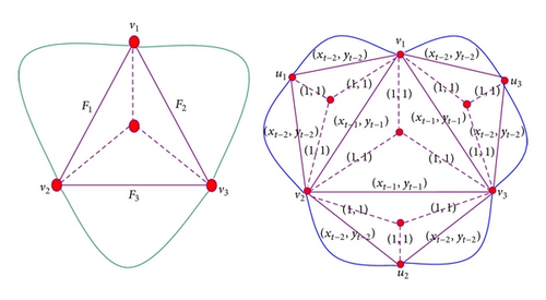
In this paper, we propose a generation algorithm of a deterministic planar network model. And we analyze its topological properties; the results show that our model has a discrete exponential degree distribution, high clustering, and small diameter, which appears small-world effect. In addition, it is known to us that the number of spanning trees is an important quantity characterizing the reliability of a network. Generally, the number of spanning trees in a network can be obtained by directly calculating a related determinant corresponding to the network. However, for a large network, evaluating the relevant determinant is intractable [18]. Therefore, we propose a generic linear algorithm to count the number of spanning trees of the general planar networks. Using the algorithm, we derive analytically the exact numbers of spanning trees in the planar networks. Based on the number of spanning trees, we determine the entropy of its spanning trees.

2. Network Construction

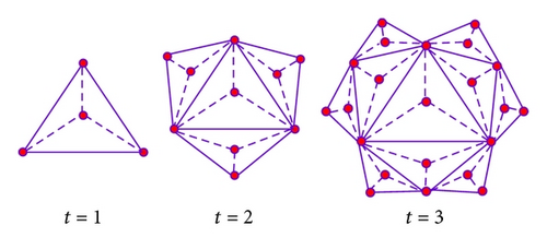
The studied network is constructed in an iterative way. We denote the network after t steps by M(t). Then, the network at step t is built as follows. For t = 1, M(1) is a complete graph with 4 nodes. For t ≥ 2, M(t) is obtained from M(t − 1) by replacing each existing iterative edge in M(t − 1) with M(1). The process is repeated till the desired graph order is reached; see Figure 1.

Details are in the caption following the image — **Figure 1**
Open in figure viewer PowerPoint

(Color online) construction of the deterministic planar network M(t), showing three steps of the iterative progress. The solid links are iterated links; the dashed links are noniterated links.

Now, we compute the order and size of M(t). Let L_v(t), L_e(t), and L_i(t) denote, respectively, the set of vertices, edges, and iterative edges introduced at step t, while V(t) and E(t) are the set of vertices and edges of the graph M(t). Notice that, at each iteration, an iterative edge is replaced by two new iterative edges and three noniterative edges. Therefore, |L_i(t)| = 2|L_i(t − 1)|, and |L_i(t)| = 3 · 2^t−1 (t ≥ 1). As each iterative edge introduces at the next iteration two new vertices and five new edges, we have |L_v(t)| = 2|L_i(t − 1)| = 3 · 2^t−1 (t ≥ 2) and |L_e(t)| = 5|L_i(t − 1)| = 15 · 2^t−2 (t ≥ 2). As L_i(1) = 3, |L_v(t)| = 4 and |L_e(t)| = 6. Thus,

()

The average degree is then

()

Obviously, for large t, it is approximately equal to 5.

3. Relevant Characteristics of the Deterministic Small-World Network

In the following, we concentrate on the degree distribution, clustering coefficient, and diameter.

3.1. Degree Distribution

The degree is the simplest and the most intensively studied characteristic of an individual node. The degree of a node i is the number of edges in the whole network connected to i. The degree distribution P(k) is defined as the probability that a randomly selected node has exactly k edges.

Let k_i(t) be the degree of node i at step t. All nodes can be divided into two categories. (i) Interior nodes; for those nodes that only connect to noniterative edges, their degree is always equal to 3. (ii) Noninterior nodes; one can see that at any iteration, a iterative edge is replaced by two new iterative edges and three new noniterative edges, so the degree of noninterior nodes is added 4 at each iteration. Thus, the degree k_i(t) of a node i satisfies the relation k_i(t + 1) = k_i(t) + 4. Then, k_i(t) = 4t − 1. And we have

()

Let t_i be the step at which a node i is created, then k_i(t_i) = 3, and hence, for noninterior nodes, we have

()

Therefore, the degree spectrum of the present network is a series of discrete values: at step t, the number of nodes of degree k = 3,7, 11, …, 4t − 9,4t − 5,4t − 1, equals 9 · 2^t−2 − 2, |L(t − 2)|, |L(t − 3)|, …, |L(2)|, |L(1)|, |L(1)|, respectively. Other values of degree are absent in the spectrum. Due to the discreteness of this degree spectrum, it is convenient to obtain its cumulative degree distribution [18]; that is,

()

Using (5), we have

. Hence,

()

Obviously, when the size of the network is large, the degree distribution P_cum(k) = 2^{(3/4)−(k/4)} is an exponential of a power of degree k.

3.2. Clustering Coefficient

Clustering coefficient is another significant property of a network, which provides a measure of the local structure within the network. The most immediate measure of clustering is the clustering coefficient C_i for every node i. By definition, clustering coefficient C_i of a node i is the ratio of the total number E_i of edges that actually exist between all k_i its nearest neighbors and the number k_i(k_i − 1)/2 of all possible edges between them; that is, C_i = 2E_i/[k_i(k_i − 1)]. The clustering coefficient C_t of the whole network is the average of all individual s. For this network, we can obtain the exact expression of the clustering coefficient C_t. By construction, for any given node u having a degree k, there are E_u = 3 · (k − 1)/2 links that actually exist among the neighbor nodes. So, one can see that there is a one-to-one corresponding relation between the coefficient C(k) of the node and its degree k: C(k) = 3/k. This expression indicates that the local clustering scales as C(k) ~ k⁻¹.

Clearly, the number of nodes of degree k = 3,7, 11, …, 4t − 9,4t − 5,4t − 1, equals 9 · 2^t−2 − 2, |L(t − 2)|, |L(t − 3)|, …, |L(2)|, |L(1)|, |L(1)|, respectively. The clustering coefficient C_t is given by the following:

()

For infinite t, C_t approaches to a constant value of 0.8309, so the clustering is high.

3.3. Diameter

Besides degree distribution and clustering coefficient, average path length (APL) is another important parameter to characterize a network. APL is defined as the average number of edges along the shortest paths for all possible pairs of network nodes. People have found the small-world phenomenon in most real-life networks that behave with a short APL. For most network models, it is hard to obtain the analytic solution of APL. To demonstrate the short distance between any pair of nodes, we can adopt another parameter that is defined as the maximal communication delay in the network. If a network has a small diameter, then this network is undoubtedly with a short APL [19]. For the network proposed, we denote the diameter at iteration t as D(t). According to Figure 1, we can clearly know that D(1) = 1 and D(2) = 2. At each iteration, one can see that the diameter always lies between a pair of newly created nodes at this iteration because at each iterative edge we paste a complete graph M(1), so the diameter for the network proposed has the following simple formula, D(t) = t.

Notice that the logarithm value of total number of nodes |V(t)| is approximately equal to tln 2 for large t. Thus, the diameter grows logarithmically with the number of nodes and the average path length increases more slowly than ln |V(t)|.

Based on the above discussions, our model is a deterministic small-world network because it is a sparse one with high clustering and short diameter, which satisfies the necessary property for small-world network.

4. Spanning Trees in the Network

In this section, we investigate the number of spanning trees in this network. Our aim is to derive the exact formula for the number of spanning trees and determine its entropy.

Let M(t) be a planar graph generated by t steps. Since M(t) is symmetry, suppose that the edges v₁v₂, v₁v₃, and v₂v₃ are weighted by (x_t−1, y_t−1), where x_t−1 denote the number of spanning trees of the subgraph F₁ and y_t−1 denote the number of spanning forests of the subgraph F₁ with two components such v₁ and v₂ belong to distinct components. Let N_ST(t) be the number of spanning trees of M(t). Figure 3 gives all spanning trees of M(1) and Figure 4 gives all spanning forests with two components. Then, by Figure 2, we have

()

According to Figures 2, 3, and 4, we obtain the recursion relations between x_t−1 and x_t−2 as follows:

()

Let a_t−1 = x_t−1/y_t−1, by (10) it follows that

()

with the initial condition a₀ = 1. So, we get

()

By (9),

()

Substituting (11) and (12) with (13), we have

()

From (14), together with (1), we determine the entropy of the number of spanning trees—an important quantity characterizing network structure—for M(t) as the limiting value [20, 21]:

()

The obtained entropy of spanning trees in M(t) can be compared to those found in other networks. In the pseudofractal fractal web [22], the entropy is 0.8959, a value less than 1, for the square lattice [23] and the two-dimensional Sierpinski gasket [24], their entropy of spanning trees is 1.16624 and 1.0486, respectively, and for the fractal scale-free lattice [25], the entropy is 1.0397. And all of them have the same average degree of 4. While in Apollonian network [26] having the average degree of 6, the entropy is 1.3540, the entropy of our model with average degree of 5 is between them.

5. Conclusion

In conclusion, we have investigated a simple model, which is constructed in a deterministic way. Then, we have presented an exhaustive analysis of many properties of the considered model and obtained the analytic solutions for most of the topological features, including degree distributions, clustering coefficient, and diameter. Finally, according to the special structure, we give a general algorithm to count the number of spanning trees of this model. Using the algorithm, we obtained entropies of spanning trees.

Conflict of Interests

The authors declare that there is no conflict of interests regarding the publication of this paper.

Acknowledgments

This research supported by the National Science Foundation of China (nos. 61164005 and 60863006), the National Basic Research Program of China (no. 2010CB334708), and Program for Changjiang Scholars and Innovative Research Team in University (no. IRT1068).

References

1 Albert R. and Barabási A. L., Statistical mechanics of complex networks, Reviews of Modern Physics. (2002) 74, no. 1, 47–97, https://doi.org/10.1103/RevModPhys.74.47, ZBL1205.82086.
10.1103/RevModPhys.74.47
CAS PubMed Web of Science® Google Scholar
2 Dorogovtsev S. N. and Mendes J. F. F., Evolution of networks, Advances in Physics. (2002) 51, no. 4, 1079–1187, 2-s2.0-0036610173, https://doi.org/10.1080/00018730110112519.
10.1080/00018730110112519
Web of Science® Google Scholar
3 Newman M. E. J., The structure and function of complex networks, SIAM Review. (2003) 45, no. 2, 167–256, 2-s2.0-0038718854, https://doi.org/10.1137/S003614450342480, ZBL1029.68010.
10.1137/S003614450342480
Web of Science® Google Scholar
4 Boccaletti S., Latora V., Moreno Y., Chavez M., and Hwang D.-U., Complex networks: structure and dynamics, Physics Reports. (2006) 424, no. 4-5, 175–308, 2-s2.0-31344474880, https://doi.org/10.1016/j.physrep.2005.10.009.
10.1016/j.physrep.2005.10.009
Web of Science® Google Scholar
5 Zhang Z., Lin Y., Gao S., Zhou S., and Guan J., Average distance in a hierarchical scale-free network: an exact solution, Journal of Statistical Mechanics. (2009) 2009, no. 10, 2-s2.0-71049194329, https://doi.org/10.1088/1742-5468/2009/10/P10022, P10022.
10.1088/1742-5468/2009/10/P10022
Web of Science® Google Scholar
6 Zhang Z. Z., Zhou S. G., and Fang J. Q., Recent progess of deterministic models of complex networks, Complex Systems and Complexity Science. (2008) 16723813.
Google Scholar
7 Dorogovtsev S. N. and Mendes J. F. F., Scalling behavior of developing and decaying networks, Europhysics Letters. (2000) 52, no. 1, https://doi.org/10.1209/epl/i2000-00400-0.
10.1209/epl/i2000-00400-0
Google Scholar
8 Kleinberg J. M., Navigation in a small world, Nature. (2000) 406, no. 6798, 2-s2.0-0343441557, https://doi.org/10.1038/35022643.
10.1038/35022643
PubMed Web of Science® Google Scholar
9 Ozik J., Hunt B. R., and Ott E., Growing networks with geographical attachment preference: emergence of small worlds, Physical Review E. (2004) 69, no. 2, 026108–5, 2-s2.0-37649026986, https://doi.org/10.1103/PhysRevE.69.026108, 026108.
10.1103/PhysRevE.69.026108
Web of Science® Google Scholar
10 Barabási A.-L., Ravasz E., and Vicsek T., Deterministic scale-free networks, Physica A. (2001) 299, no. 3-4, 559–564, 2-s2.0-0035887972, https://doi.org/10.1016/S0378-4371(01)00369-7, ZBL0972.57003.
10.1016/S0378-4371(01)00369-7
Web of Science® Google Scholar
11 Watts D. J. and Strogatz S. H., Collective dynamics of small world network, Nature. (1998) 393, no. 6684, 440–442, 2-s2.0-0032482432, https://doi.org/10.1038/30918.
10.1038/30918
CAS PubMed Web of Science® Google Scholar
12 Zhang Z., Rong L., and Guo C., A deterministic small-world network created by edge iterations, Physica A. (2006) 363, no. 2, 567–572, 2-s2.0-33644859121, https://doi.org/10.1016/j.physa.2005.08.020.
10.1016/j.physa.2005.08.020
Web of Science® Google Scholar
13 Newman M. E. J. and Watts D. J., Renormalization group analysis of the small-world network model, Physics Letters A. (1999) 263, no. 4–6, 341–346, 2-s2.0-0347334779, https://doi.org/10.1016/S0375-9601(99)00757-4, ZBL0940.82029.
10.1016/S0375-9601(99)00757-4
CAS Web of Science® Google Scholar
14 Newman M. E. J. and Watts D. J., Scaling and percolation in the small-world network model, Physical Review E. (1999) 60, no. 6, 7332–7342, 2-s2.0-0033487710, https://doi.org/10.1103/PhysRevE.60.7332.
10.1103/PhysRevE.60.7332
CAS PubMed Web of Science® Google Scholar
15 Kasturirangan R., Multiple Scales in Small-World Graphs, 1999, no. AI Lab Memo. 1663, Massachusetts Institute of Technology.
Google Scholar
16 Erdös P. and Rényi A. R., On random graphs I, Publicationes Mathematicae. (1959) 6, 290–297, ZBL0092.15705.
10.5486/PMD.1959.6.3-4.12
Google Scholar
17 Erdös P. and Rényi A. R., On the evolution of random graphs, Publication of the Mathematical Institute of the Hungarian Academy of Sciences. (1960) 5, 17–61, ZBL0103.16301.
Google Scholar
18 Xiao Y. Z. and Zhao H. X., New method for counting the numberof spanning trees in a two-tree network, Physica A. (2013) 392, 4576–4583, https://doi.org/10.1016/j.physa.2013.05.007.
10.1016/j.physa.2013.05.007
Web of Science® Google Scholar
19 Lu Z.-M. and Guo S.-Z., A small-world network derived from the deterministic uniform recursive tree, Physica A. (2012) 391, no. 1-2, 87–92, 2-s2.0-80054017215, https://doi.org/10.1016/j.physa.2011.08.002.
10.1016/j.physa.2011.08.002
Web of Science® Google Scholar
20 Burton R. and Pemantle R., Local characteristics, entropyand limit theorems for spanning trees and domino tilingsvia transfer-impedances, Annals of Probability. (1993) 21, https://doi.org/10.1214/aop/1176989121.
10.1214/aop/1176989121
Google Scholar
21 Lyons R., Asymptotic enumeration of spanning trees, Combinatorics Probability and Computing. (2005) 14, no. 4, 491–522, 2-s2.0-23844524256, https://doi.org/10.1017/S096354830500684X, ZBL1076.05007.
10.1017/S096354830500684X
Web of Science® Google Scholar
22 Zhang Z. Z., Liu H. X., Wu B., and Zhou S. G., Enumeration of spanning trees in a pseudofractal scale-free web, Europhysics Letters. (2010) 90, no. 6, 680029, https://doi.org/10.1209/0295-5075/90/68002.
10.1209/0295-5075/90/68002
Google Scholar
23 Wu F. Y., Number of spanning trees on a lattice, Journal of Physics A. (1977) 10, no. 6, article 4, L113–L115, 2-s2.0-0000033790, https://doi.org/10.1088/0305-4470/10/6/004.
10.1088/0305-4470/10/6/004
Google Scholar
24 Chang S.-C., Chen L.-C., and Yang W.-S., Spanning trees on the Sierpinski gasket, Journal of Statistical Physics. (2007) 126, no. 3, 649–667, 2-s2.0-33847185591, https://doi.org/10.1007/s10955-006-9262-0, ZBL1110.82007.
10.1007/s10955-006-9262-0
Web of Science® Google Scholar
25 Zhang Z., Liu H., Wu B., and Zou T., Spanning trees in a fractal scale-free lattice, Physical Review E. (2011) 83, no. 1, 2-s2.0-79951705659, https://doi.org/10.1103/PhysRevE.83.016116, 016116.
10.1103/PhysRevE.83.016116
Web of Science® Google Scholar
26 Lin Y., Wu B., Zhang Z., and Chen G., Counting spanning trees in self-similar networks by evaluating determinants, Journal of Mathematical Physics. (2011) 52, no. 11, 2-s2.0-82855170971, https://doi.org/10.1063/1.3659687, 113303, ZBL1272.05187.
10.1063/1.3659687
Web of Science® Google Scholar

All articles

A New Class of the Planar Networks with High Clustering and High Entropy

Abstract

1. Introduction

2. Network Construction