Equilibrium Asset and Option Pricing under Jump-Diffusion Model with Stochastic Volatility
Abstract
We study the equity premium and option pricing under jump-diffusion model with stochastic volatility based on the model in Zhang et al. 2012. We obtain the pricing kernel which acts like the physical and risk-neutral densities and the moments in the economy. Moreover, the exact expression of option valuation is derived by the Fourier transformation method. We also discuss the relationship of central moments between the physical measure and the risk-neutral measure. Our numerical results show that our model is more realistic than the previous model.
1. Introduction
Option pricing problem is one of the predominant concerns in the financial market. Since the advent of the Black-Scholes option pricing formula in [1], there has been an increasing amount of literature describing the theory and its practice. Due to drawbacks of the Black-Scholes model which cannot explain numerous empirical facts such as large and sudden movements in prices, heavy tails, volatility clustering, the incompleteness of markets, and the concentration of losses in a few large downward moves, many option valuation models have been proposed and tested to fit those empirical facts. Jump-diffusion models with stochastic volatility could overcome these drawbacks of the Black-Scholes model in [2–21]. Based on those advantages, in this paper, we focus on studying the jump-diffusion model with stochastic volatility.
Different from the Black-Scholes framework, we use jump diffusion to describe the price dynamics of underlying asset. The market of our model is incomplete; that is, it is not possible to replicate the payoff of every contingent claim by a portfolio, and there are several equivalent martingale measures. How to choose a consistent pricing measure from the set of equivalent martingale measures becomes an important problem. This means that we need to find some criteria to determine one from the set of equivalent martingale measures in some economically or mathematically motivated fashion. A unique martingale measure was found by various researchers via using optimal criteria, for instance, minimal martingale criterion, minimal entropy martingale criterion, and utility maximization criterion [22–31].
General equilibrium framework method is also a popular method to deal with the option pricing in an incomplete market. General equilibrium framework is initially introduced by Lucas Jr. (1978) [32], Cox et al. (1985) [33] and developed by Vasanttilak and Lee (1990) [34], Pan (2002) [35], Liu and Pan (2003) [36], Liu et al. (2005) [37], Bates (2008) [38], Santa-Clara and Yan (2004) [12], and Zhang et al. (2012) [6]. They assumed that there is a representative investor who wants to maximize an objective function in a rational expectations economy where there are one risk-free asset and one risky asset. When the market is clear, the representative investor takes all money into the risky asset. In this paper, we build a general equilibrium model which is the same as that due to Santa-Clara and Yan (2004) [12]. Under this model, we obtain an exact expression of the equity premium and the pricing kernel in a general equilibrium economy. This can be regarded as a great contribution to the literature.
The pricing kernel which acts like the physical and risk-neutral densities and moments in the economy is also a vitally important problem in mathematical finance. In some constant volatility models with jump diffusions, Pan (2002), Liu and Pan (2003), and Liu et al. (2005) [35–37] derived the pricing kernel with some restrictions of jump sizes in a general equilibrium setting. Recently, Zhang et al. (2012) [6] presented an analytical form for the pricing kernel without any distributional assumption on the jumps. In this paper, we extend the results of Zhang et al. (2012) to the pricing kernel with stochastic volatility.
Duffie et al. (2000) [10] and Chacko and Das (2002) [39] presented a transform analysis to price the valuation of options for affine jump diffusions with stochastic volatility. Lorig and Lozano-Carbasse (2013) [21] studied option pricing in exponential Lévy-type models with stochastic volatility and stochastic jump intensity. Lewis (2008) [8] used Fourier transformation methods to obtain the transform-based solution of option price. In this paper, we employ the Fourier transformation method to get the exact expression of European options.
Finally, we get the relationship of central moments between the physical measure and the risk-neutral measure which can help us to study the negative variance risk premium, the implied volatility smirk, and the prediction of realized skewness. Some relevant work has been done by Bakshi et al. (2003) [13], Carr and Wu (2009) [14], and Neuberger (2012) [15]. However, to the best of our knowledge, except for Zhang et al. (2012) [6], there is no literature studying this relationship. In this paper, we extend it to a stochastic volatility case. This can be regarded as another contribution to the literature.
The rest of the paper is organized as follows. In Section 2, we present our jump-diffusion model with stochastic volatility. In Section 3, we study the equity premium in a general equilibrium economy. The option pricing and the relationship of central moments between the physical measure and the risk-neutral measure are studied in Section 4. Numerical results and conclusions are shown in Sections 5 and 6, respectively.
2. Our Model
- (i)
A Bond whose price Pt at time t is given by
() - (ii)
A Stock whose price St at time t is given by
()
3. Equity Premium
The equity premium is very important for option pricing in general equilibrium framework. Following the idea of Santa-Clara and Yan (2004) [12] and Zhang et al. (2012) [6], we obtain the equilibrium equity premium by modeling general equilibrium economy in the following proposition.
Proposition 1. In general equilibrium framework, the equilibrium equity premium is given by
Proof. From the optimal control problem (5), we get the Bellman equation as follows:
Equating the derivatives of the Bellman equation (9) with respect to ω to zero, we have following equation:
In equilibrium, the money market is in zero net supply. Therefore, the representative investor holds all the wealth in the stock market; that is, ω = 1. Then we can get the expression of ϕ from (11):
This system (16) and (17) can be solved explicitly. First, we solve the first ODE (16), which is the Riccati differential equation. Making the substitution
Remark 2. In the special case where there is no stochastic volatility and jumps, Vt = σ2 and ε = κ = 0, and consequently ϕ = σ2γ which is constant in Merton (1976) [2]. In the special case where there is no stochastic volatility, ε = 0, and consequently ϕ = σ2γ + λE[(1 − e−γx)(ex − 1)] which is constant in Zhang et al. (2012) [6].
4. Option Pricing
In this section, we will study the pricing kernel and the option pricing in general equilibrium framework. We first derive the pricing kernel which acts like the physical and risk-neutral densities in the economy and is the key to obtain the PDE of option price as follows.
Proposition 3. In general equilibrium framework, the pricing kernel is given in differential form by
The martingale condition, πtSt = Et[πTST], requires that the jump size y satisfies the following restriction:
Proof. To satisfy the martingale condition, πtSt = Et[πTST], from (3) and (26), we have
Remark 4. In this market, there is only one tradable asset, a stock with price St, but there are at least two dimensions of risk, diffusive risk, and jump risk. Therefore, the market is incomplete and the pricing kernel is not unique. The nonuniqueness of the pricing kernel can be justified by the fact that the distribution of jump size y in the pricing kernel can be arbitrary as long as it satisfies the martingale restriction (27). In a special case, we can choose y = −γx, as in Liu et al. (2005) [37].
Remark 5. With Proposition 3, we define a new probability measure Q:
Lemma 6. Define a new probability measure, Q*, by the following Radon-Nikodym derivative:
Proof. The change of probability measure formula gives
Since yi, i = 1,2, …i, …, n, is i.i.d. and y and x are correlated, this means that only one of the yi is correlated with x. Without loss of generality, we assume that yn is correlated with x and other yis are independent of x. Then we have
Remark 7. These results are also true in Q measure, because the difference between Q and Q* is the Brownian motion that is independent of the jumps.
Now, we consider a European call written on the stock price St at time t. The option has a payoff function (ST − K) + at time T. Its price is denoted as c(St, Vt, t) at time t. We derive a PDE which c(St, Vt, t) has to satisfy in the following proposition.
Proposition 8. In general equilibrium framework, the price of European call option satisfies the following PDE:
Proof. First, we rewrite the stock with continue part and jump part:
Remark 9. The stock process (2) in a risk-neutral measure Q can be written as
Furthermore, we also can understand λQ = λE(ey) by
Remark 10. κQ = κ + (γ − ερA)ερ and θQ = (κθ/(κ + (γ − ερA)ερ)) are similar forms in Heston (1993) [40].
Following the approach of Lewis (2000) [8], we will derive the pricing formula in a risk-neutral measure Q from the PDE.
Proposition 11. In general equilibrium framework, the pricing formula is given by
Proof. We denote X = ln S and g(X, V, t): = c(eX, V, t) = c(S, V, t); then, the PDE (36) can be rewritten as
Denote k = kr + iki; the inverse Fourier transform is given by
Denote h ≡ e(1+ik)rτG; the PDE (58) can be rewritten as
According to the study of Lewis (2000) [8], to solve the PDE (59) with the initial condition (60), it is enough to solve the same equation with the initial value being equal to one. We call this solution fundamental transform and denote it h(k, V, τ) which satisfies following equation by:
Denoting H(V, τ): = h(k, V, τ), then, the PDE (61) can be rewritten as
We guess that a solution of (63) is as the following form:
This leads to a system of two ODEs:
This system can be solved explicitly. First, we solve the first ODE (65), which is the Riccati differential equation. Making the substitution
A general solution of (68) has the form
Then, the solution of the second ODE (66) is
Note. Although the pricing formula (40) contains a complex integral, the result is real.
With the European option price being well understood, we study the relations between the physical and risk-neutral densities and moments which can help us to study the negative variance risk premium, the implied volatility smirk, and the prediction of realized skewness. In this paper, we extend the results about those relations in [6] to a stochastic volatility case.
Proposition 12. The risk-neutral density of the continuously compounded return within τ = T − t, Rτ = ln ST/St, St given in (38), is given by
The physical density is given by
Proof. We denote the corresponding probability function Φ = Prob(ST ≤ K), and Φ also satisfies the PDE (36) with a different boundary condition . Under the Fourier transform, this boundary condition becomes (Kik/ik). Solving the PDE (36) under this new boundary condition, we have
We denote the stock return between time t and T by R so that K = SeR; then we can differentiate Φ with respect to R to get the density function φQ(Rτ∣V, τ). We find that the parameters of the physical stock price process in (2) are the same those of risk-neutral stock price process in (50); then the parameters of φ(Rτ∣V, τ) are just removed by the superscript ·Q.
Now we compute the first moment, second, third, and fourth central moments of the continuously compounded return in the physical measure. There are at least two methods to solve the problem of how to compute central moments.
One method is using the Rτ’s characteristic function to calculate the nth moment of Rτ. Since
Although this method is very straightforward, it is too complicated to calculate the integration. We introduce another way to obtain the central moments by a direct calculation.
From (3), we have
Then, the first moment of the continuously compounded return in the physical measure can be easy to be obtained:
Define the first central moment, second, third, and fourth central moments in the physical measure of random number x as , , , and .
From (2) we have
Remark 13. If , where σ2 is constant, our results will degenerate into Proposition 3.19 by Zhang et al. (2012) [6].
We denote , as the skewness and kurtosis in risk-neutral measure, respectively. Skewness and kurtosis are very important for asset pricing. For example, Bakshi et al. (2003) [13] concluded that variations in the risk-neutral skew were instrumental in explaining the differential pricing of individual equity options and found that less negatively skewed stocks have flatter smiles. From Proposition 12, we easily obtain the following three corollaries about skewness and kurtosis.
Corollary 14. The skewness and kurtosis in physical measure are given by
Corollary 15. For jump size x, the first moment and the second, third, and fourth central moments in the physical measure are given by
Proof. To compute central moments in the physical measure, we have , , , , and .
Corollary 16. For small risk aversion coefficient, one has the following relationship between the third central moments in the neutral-risk measure and in the physical measure:
Proof. From Corollary 15, for small risk aversion coefficient x, we have
5. Numerical Results
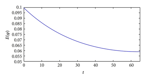
If we assume that other parameter values in our model are k = 0.03, V0 = 0.1, ε = 0.1, and ρ = −0.25, we will find that the expectation of ϕ tends to 0.6 from Figure 1, which is consistent with above analysis.

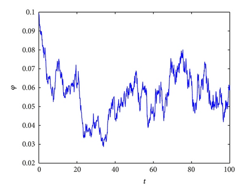
One path of ϕ is given in Figure 2.

In realistic world, the risk premium is stochastic. For example, Figure 1a and Figure 5 in Graham and Harvey (2012) show that risk premium follows mean-reverting stochastic process in [41]. Thus, our model is more realistic than that in [6].
6. Conclusions
We successfully extend the model in [6] and obtain more general results. First, the equilibrium equity premium in general equilibrium framework links not only the jump risk but also the stochastic volatility risk. Moreover, the pricing kernel with stochastic volatility is shown in this paper. We employ the Fourier transformation method to obtain the exact expression of option price. Next, we get the relationship of central moments between the physical measure and risk-neutral measure. It is a vitally crucial problem in financial area. Our numerical results show that our model is more realistic than the one in [6].
Acknowledgment
This work is supported by the Fundamental Research Funds for the Central Universities (JBK130401).


