Asymptotic Behavior of a Viscoelastic Fluid in a Closed Loop Thermosyphon: Physical Derivation, Asymptotic Analysis, and Numerical Experiments
Abstract
Fluids subject to thermal gradients produce complex behaviors that arise from the competition with gravitational effects. Although such sort of systems have been widely studied in the literature for simple (Newtonian) fluids, the behavior of viscoelastic fluids has not been explored thus far. We present a theoretical study of the dynamics of a Maxwell viscoelastic fluid in a closed-loop thermosyphon. This sort of fluid presents elastic-like behavior and memory effects. We study the asymptotic properties of the fluid inside the thermosyphon and the exact equations of motion in the inertial manifold that characterizes the asymptotic behavior. We derive, for the first time, the mathematical derivations of the motion of a viscoelastic fluid in the interior of a closed-loop thermosyphon under the effects of natural convection and a given external temperature gradient.
1. Introduction
Instabilities and chaos in fluids subject to temperature gradients have been the subject of intense work for its applications in engineering and in atmospheric sciences. In such sort of systems, the fluid displays nontrivial behaviors (as turbulence or the formation of convective rolls) when subject to a heating that competes with buoyancy effects. A traditional approach that goes back to the pioneering work by Lorenz consists of the study of the system under some simplifications. Another approach is to study the controlled setups that capture the underlying complexity of the full system, being a thermosyphon one of those simpler cases [1].
In the engineering literature, a thermosyphon is a device composed of a closed-loop pipe containing a fluid where some soluble substance has been dissolved [2, 3]. The motion of the fluid is driven by the action of several forces such as gravity and natural convection. The flow inside the loop is driven by an energetic balance between thermal energy and mechanical energy. The interest on this system comes both from engineering and as a toy model of natural convection (for instance, to understand the origin of chaos in atmospheric systems).
Thus far, all the works on thermosyphons analyze the behavior of a Newtonian fluid inside the loop, consequently neglecting elastic effects in the system coming from either the fluid itself or the elastic walls of the loop. However, many interesting fluids are known to behave slightly different from the common (Newtonian) fluids in terms of their response to an applied stress and are commonly referred to as viscoelastic. Among them, it is worth emphasizing volcanic lavas, snow avalanches, flowing paint, or biological mucosas membranes.
Here, we consider a thermosyphon model in which the confined fluid is viscoelastic. This has some a priori interesting peculiarities that could affect the dynamics with respect to the case of a Newtonian fluid. On the one hand, the dynamics has memory and so its behavior depends on the whole past history, and, on the other hand, at small perturbations the fluid behaves like an elastic solid and a characteristic resonance frequency could, eventually, be relevant (e.g., consider the behavior of jelly or toothpaste).
The simplest approach to viscoelasticity comes from the so-called Maxwell constitutive equation [4]. In this model, both Newton’s law of viscosity and Hooke’s law of elasticity are generalized and complemented through an evolution equation for the stress tensor, σ.
The derivation of the thermosyphon equations of motion is similar to that in [2, 3]. The simplest way to incorporate (2) is by differentiating (1) with respect to time and replacing the resulting time derivative of σ with (2). This way to incorporate the constitutive equation allows to reduce the number of unknowns (we remove σ from the system of equations) at the cost of increasing the order of the time derivatives to second order.
The model we will take into consideration forms an ODE/PDE system for the velocity v(t), the distribution of the temperature T(t, x) of the fluid into the loop, (5) with ν ≥ 0, where denotes integration along the closed path of the circuit. The function f describes the geometry of the loop and the distribution of gravitational forces [2, 3]. Note that ∮f = 0.
The system of (5) is not a trivial extension of the Newtonian model in [11] due to the first term in the differential equation for the velocity. Specifically, the addition of a term proportional to the second derivative of v is singular, in the sense that it changes qualitatively the character of the equations. The implications of this singular perturbation cannot be ascertained using a standard boundary layer analysis (see the Appendix for details). So a complementary theoretical and numerical approach is mandatory.
We assume that G(v) which specifies the friction law at the inner wall of the loop is positive and bounded away from zero. This function has been usually taken to be G(v) = G, a positive constant for the linear friction case [2] (Stokes flow), or G(v) = |v| for the quadratic law [12, 13], or even a rather general function given by , where Re is the Reynolds number, Re = ρvL/μ. Here we will consider a general function of the velocity assumed to be large [9, 14]. The functions G, f, l, and h incorporate relevant physical constants of the model, such as the cross-sectional area, D, the length of the loop, L, and the Prandtl, Rayleigh or Reynolds number; see [9]. Here, we consider Newton’s linear cooling law l(v)(Ta − T) where l represents the heat transfer law across the loop wall, and is a positive quantity depending on the velocity, and Ta is the (given) ambient temperature distribution, see [3, 5, 9, 10].
Hereafter, we consider G and l as continuous functions, such that G(v) ≥ G0 > 0, and l(v) ≥ l0 > 0, for G0 and l0 positive constants.
- (i)
To obtain the system of (5) governing a closed loop thermosyphon model with a viscoelastic fluid and to study the asymptotic behavior of this system which is a generalization of the previous model [11]. Thus, although the dynamics of viscoelastic fluids has been extensively studied in the engineering literature, it has scarcely been considered in the applied mathematics community.
- (ii)
To present an analysis beginning with the well-posedness and boundedness of solution. The existence of an attractor and an inertial manifold is shown and an explicit reduction to low-dimensional systems is obtained. It is noteworthy that we are able to obtain an exact finite-dimensional reduction (87) that may have a much lower number of degrees of freedom.
- (iii)
To provide a detailed numerical analysis of the behavior of acceleration, velocity, and temperature which includes a thorough study of the various behaviors of the system for different values of viscoelastic fluid and ambient temperature distribution.
- (iv)
The numerical analysis will show that viscoelasticity induces a chaotic behavior that is not captured by a boundary layer analysis (that would predict the same qualitative behaviors as in the original model in [11] see the Appendix for details) being the new (nontrivial) emergent behaviors induced by the viscoelasticity worth characterizing.
2. Well-Posedness and Boundedness: Global Attractor
2.1. Existence and Uniqueness of Solutions
In this section we prove the existence and uniqueness of solutions of the thermosyphon model (5).
First, we observe that for ν ≥ 0, if we integrate the equation for the temperature along the loop taking into account the periodicity of T, that is, ∮(∂T/∂x) = ∮(∂2T/∂x2) = 0, we have (d/dt)(∮T) = l(v)(∮Ta − ∮T). Therefore, ∮T → ∮Ta exponentially as time goes to infinity for every ∮T0.
Thus, with w = dv/dt, we get (w, v, τ) verifying the system (5) with τa, τ0 replacing Ta, T0, respectively, and now ∮τ = ∮τa = ∮τ0 = ∮f = 0. Therefore, hereafter we consider the system (5) where all functions have zero average.
Also, if ν > 0, the operator νA = −ν(∂2/∂x2), together with periodic boundary conditions, is an unbounded, self-adjoint operator with compact resolvent in that is positive when restricted to the space of zero average functions . Hence, the equation for the temperature T in (5) is of parabolic type for ν > 0.
2.1.1. The Case with Diffusion: ν > 0
Using the results and techniques of sectorial operator of [15], we obtain Theorem 1.
Theorem 1. We assume that H(r) = rG(r) and l(v) are locally Lipschitz, , , and l(v) ≥ l0 > 0. Then, given , there exists a unique solution of (5) satisfying
Proof. We cover several steps.
Step 1. We prove the local existence and regularity. This follows easily from the variation of constants formula of [15]. In order to prove this we write the system as (9), and we have
Using H(v) = G(v)v and l(v) being locally Lipschitz together with and , we will prove the nonlinear terms, F1(w, v, T) = −(1/ɛ)G(v)v + (1/ɛ)∮Tf, F2(w, v, T) = w, and F3(w, v, T) = −v(∂T/∂x) + l(v)(Ta − T) and satisfy , , and ; that is, F : 𝒴 ↦ 𝒴−1/2 is well defined, Lipschitz, and bounded on bounded sets. It is possible to prove this by considering . In order to prove these properties of the nonlinearity F, let Ui = (wi, vi, Ti) t, and we note that
Therefore, using the techniques of variations of constants formula of [15], we obtain the unique local solutions (w, v, T) ∈ C([0, τ], 𝒴) of (8) which are given by
with H(r) = H(v(r)),
Step 2. Now, we prove the solutions of (8) for every time t ≥ 0.
To prove the global existence, we must show that the solutions are bounded in norm on finite time intervals. First, to obtain that the norm of T is bounded in finite time, we note that multiplying the equations for the temperature by T in and integrating by parts, we have:
Using Cauchy-Schwartz and the Young inequality and then the Poincaré inequality, since ∮T = 0 together with π2 is the first nonzero eigenvalue of A = −∂2/∂x2 in , we obtain
Now, we note that differentiating the second equation of (5) with respect to x, we obtain the same equations for ∥∂T/∂x∥, and considering now ∥∂Ta/∂x∥, we obtain
Thus, we show that the norm of T in remains bounded in finite time. Then, using ∥T∥ bounded for finite time, we prove that |w(t)| and |v(t)| remain bounded in finite time and we conclude.
2.1.2. The Case with No Diffusion: ν = 0
To prove the system is well posed, we use the techniques from [16] considering the same transport equation for temperature in different thermosyphon models as [6–8, 10, 16].
We note that for and since in this space the translations are continuous isometries, (27) defines a continuous function of time with values in this space. Although we restrict ourselves to , many other choices of space are possible for solving problem (26). In fact any Banach space of 1-periodic functions of x having zero mean and in which translations are continuous isometries can be used as an “admissible space” X; see [16]. In particular are admissible spaces between others. Then, we can prove Lemma 2.
Lemma 2. Let τ > 0, fix v ∈ C[0, τ], and assume that T0, Ta ∈ X where X is an “admissible space”; see [16], in particular . Then, the function given in (27), Tv ∈ C([0, τ], X), is an integral solution of the PDE which is satisfied only if T0 and Ta are differentiable. In particular, if , then Tv is continuous with values in and satisfies the PDE as an equality in , a.e. in time. Moreover, (27) satisfies the following properties:
- (i)
(29)
- (ii)
if there exist positive constants cd, d = a and d = 0 such that T0, Ta satisfy for all k, then Tv satisfies
(30) -
positive constant independent on time;
- (iii)
we assume that and there exist positive constants cd, d = a and d = 0 such that T0, Ta satisfy for all k. If we also assume that vi, i = 1,2 are continuous in t ∈ [0, τ], then
(31) -
K is a positive constant, and .
Theorem 3. Assume that G(v)v is locally Lipschitz, , , and w0, v0 ∈ ℝ2. Then there exists a unique solution of (26) satisfying
Proof. As noted earlier, we need to solve the fixed point problem
From (29) in Lemma 2 for Tv, we have ∥Tv∥ ≤ max{∥T0∥∥Ta∥}, and this, together with the local Lipschitz property of G(v)v shows that for fixed M, ℱ(ℳ) ⊂ ℳ if L is sufficiently small.
To show that ℱ is a contraction, it is clear that we must prove some Lipschitz dependence on ∮Tvf with respect to v ∈ W.
First, we note that from , then verify (30), that is, for all k with d = 0, a, and given vi ∈ W, again from (31) in Lemma 2, we have
To prove the global existence, it is sufficient to prove that (w(t), v(t)) is bounded on finite time intervals, since from
But again from (29) together with (18) and (19), we obtain boundedness on finite time intervals and global existence follows.
As noted earlier, if , then T satisfies the PDE equation as an equality in a.e. in time. In particular, we have .
2.2. Boundedness of the Solutions and Global Attractor
Lemma 4 (L’Hopital’s lemma). Assume that f and g are real differentiable functions on (a, b), b ≤ ∞, g′(x) ≠ 0 on (a, b) and limx→bg(x) = ∞.
- (i)
If limsupx→b(f′(x)/g′(x)) = L, then limsupx→b(f(x)/g(x)) ≤ L.
- (ii)
If liminfx→b(f′(x)/g′(x)) = L, then liminfx→b(f(x)/g(x)) ≥ L.
With this, we have Lemma 5.
Lemma 5. If one assumes that G(r) and H(r) = rG(r) satisfy the hypothesis from Theorem 1 or Theorem 3 together with (36), then
Proof. Integrating by parts we have
Remark 6. We note that the conditions (36) are satisfied for all friction functions G considered in the previous works, that is, the thermosyphon models, where G is constant or linear or quadratic law. Moreover, the conditions (36) are also true for G(s) ≈ A | s|n, as s → ∞.
Now, we use the asymptotic bounded for temperature to obtain the asymptotic bounded for the velocity and the acceleration functions.
Theorem 7. Under the previous notations and hypothesis of Theorem 1 or Theorem 3, if one assumes also that G satisfies (37) for some constant H0 ≥ 0, then one has the following.
Part (I). General case:
- (i)
(40)
-
In particular: If limsupt→∞∥T∥ ∈ ℝ, then
(41) - (ii)
If limsupt→∞∥T∥ ∈ ℝ and , then
(42)(43)
- (i)
(44)
- (ii)
(45)
- (iii)
if ,
(46)
Proof. Part (I). General case.
(i) From (8) we have that
(ii) From (47) together with Gronwall’s lemma, we get
Part (II). (i) From (23) together with (24), we get
Remark 8. First, we note that the hypothesis about the function l(v) in Theorem 7, l(v) ≤ L0 is satisfied when we consider Newton’s linear cooling law h = k(Ta − T), where k is a positive quantity; that is, l(v) = k = L0, as [18]. Moreover, this condition is also satisfied if we consider h = l(v)(Ta − T) where l(v) is a positive upper bounded function.
Second, it is important to note that we prove in the next section the existence of the global compact and connected attractor and the inertial manifold for the system (8), when we consider the general Newton’s linear cooling law without the additional previous hypothesis on l(v); but we assume that the friction function G(v) always satisfies (36).
In order to get this, we consider the Fourier expansions and observe the dynamics of each coefficient of Fourier expansions to improve the asymptotic bounded of temperature. In particular, we will prove limsupt→∞∥T(t)∥ ≤ ∥Ta∥ for every locally Lipschitz and positive function l(v) and also for every ν ≥ 0 (see (72) in Proposition 9) and for every friction function G(v) satisfying (36).
3. Asymptotic Behavior: Reduction to Finite-Dimensional Systems
The system of (5) reflects two of the main features: (i) the coupling between the modes enter only through the velocity, while diffusion acts as a linear damping term, and (ii) it is important to note in this model that we have also the nonlinear term given by Newton’s linear cooling law.
In what follows, we will exploit this explicit equation for the temperature modes to analyze the asymptotic behavior of the system and to obtain the explicit low-dimensional models.
3.1. Attractors and Inertial Manifolds
The existence of an inertial manifold does not rely, in this case, on the existence of large gaps in the spectrum of the elliptic operator but on the invariance of certain sets of Fourier modes.
A similar explicit construction was given by Bloch and Titi in [19] for a nonlinear beam equation where the nonlinearity occurs only through the appearance of the L2 norm of the unknown. A related construction was given by Stuart in [20] for a nonlocal reaction-diffusion equation.
In order to get the inertial manifold for this system, we first improve the bounds on acceleration, velocity, and temperature of the previous section for all situations with ν ≥ 0 and l(v) ≥ l0 > 0 general locally Lipschitz function under the hypotheses of Lemma 5 for some H0 ≥ 0, in particular G(v) satisfying (36).
Proposition 9. Under the previous notations, for every solution of the system (5), (w, v, T), and for every k ∈ ℤ*, one has
- (i)
(65)
- (ii)
(66)
-
and G0 a positive constant such that G(v) ≥ G0;
- (iii)
(67)
Proof. From (61), we have
We note from the previous result that we have always the upper bound for ∥T∥ and from Theorem 7 for the velocity. Therefore, we can consider L0 the upper bound for the continuous positive function l(v); we note that L0 = limsupt→∞l(v) and we prove in Proposition 10 the bound of solutions to show the influence of diffusion coefficient ν.
Proposition 10. Under the previous notations, for every solution of the system (5), (w, v, T), and for every k ∈ ℤ*, one has
Proof. Using again
In particular |ak(t)|≤(L0/(4νπ2k2 + l0)) | bk | ≤(L0/(4νπ2 + l0)) | bk| for every k ∈ ℤ* and also |ak(t)|≤(L0/(4νπ2k2 + l0)) | bk | ≤(L0/(4νπ2k2)) | bk|; that is, |ak(t)|≤(L0/4νπ2) | bk|.
Then, we also have that
Finally, we note that if L0 = limsupt→∞l(v(t)), then given δ > 0, there exists t0 such that L(v(t)) ≤ L0 + δ for every t ≥ t0, and integrating in t ≥ t0, we obtain limsupt→∞ | ak(t)|≤(L0/(4νπ2k2 + l0)) | bk | + δ, for any δ > 0, and
We note that if ν = 0, then |ak | ≤|bk | ≤(L0/l0) | bk|. If ν > 0 we observe in the numerical experiments, as ν is bigger, that the solution becomes stable or periodic.
As a consequence, we have the following result on the smoothness of the attractor of (5).
Corollary 11. (i) If |ak0 | ≤(L0/(4νπ2k2 + l0)) | bk|, then |ak(t)|≤(L0/(4νπ2k2 + l0)) | bk| for every t ≥ 0.
(ii) If 𝒜 is the global attractor in the space , then for every (w0, v0, T0) ∈ 𝒜, with , one gets
Proof. (i) From (77) we have , therefore, if |ak0 | ≤(L0/(4νπ2k2 + l0)) | bk|, then |ak(t)|≤(L0/(4νπ2k2 + l0)) | bk| for every t ≥ 0 and k ∈ ℤ*.
(ii) We note that from (i), if , then , and therefore ; that is, 𝒜 ⊂ [−M, M]×[−N, N] × 𝒞 where M, N are the upper bounds for acceleration and velocity as given in (74) and (73). But, the set 𝒞 is compact in since for any sequence {Tn} in 𝒞 we can extract a subsequence that we still denote {Tn} such that it converges weakly to a function T and such that for any k ∈ ℤ*, the Fourier coefficients verify as n → ∞, where ak is the kth Fourier coefficient of T. Therefore, 4νπ2k2 | ak | ≤|bk| and for every integer E,
Note that this result reveals in particular the asymptotic smoothing of (5). In the next result we will prove that the dynamical system induced by (8) in the phase space , m ≥ 1, has an inertial manifold. According to [21], we have the following definition.
Definition 12. Let S(t), t ≥ 0, be a nonlinear semigroup in a Banach space in 𝒴 that has a global attractor 𝒜. Then, a smooth manifold ℳ ⊂ 𝒴 is called an inertial manifold if
- (i)
ℳ is positively invariant, that is, S(t)ℳ ⊂ ℳ for every t ≥ 0;
- (ii)
ℳ contains the attractor, that is, 𝒜 ⊂ ℳ;
- (iii)
ℳ is exponentially attracting in the sense that there exists a constant δ > 0 such that for every bounded set B ⊂ 𝒴 there exists C = C(B) ≥ 0 such that
(82)
Note that from (61), if bk = 0, then the kth mode for the temperature is damped out exponentially, and therefore the space V attracts the dynamics for the temperature. This is precisely stated in the following result.
Theorem 13. Assume that and . Then, the set ℳ = ℝ2 × Vm is an inertial manifold for the flow of S(t)(w0, v0, T0) = (w(t), v(t), T(t)) in the space . Moreover, if f ∈ Vm the inertial manifold ℳ has the exponential tracking property; that is, for every , there exists (w1, v1, T1) ∈ ℳ such that if (wi(t), vi(t), Ti(t)), i = 0,1, are the corresponding solutions of (8), then (w0(t), v0(t), T0(t))−(w1(t), v1(t), T1(t)) → 0 in . In particular if K is a finite set, the dimension of ℳ is |K | + 2, where |K| is the number of elements in K.
Proof. In order to prove that ℳ is invariant, we note if k ∉ K, then bk = 0, and therefore , from (70), we get that ak(t) = 0, for every t; that is, T(t, x) = ∑k∈K ak(t)e2πkix = T1. Thus, if (w0, v0, T0) ∈ ℳ, then (w(t), v(t), T(t)) ∈ ℳ for every t, that is, invariant manifold.
We consider the decomposition in , T = T1 + T2, where T1 is the projection of T on Vm and T2 is the projection of T on the subspace generated by {e2πkix, k ∈ ℤ*∖K}; that is, T1 = ∑k∈K ake2πkix and .
From (77) taking into account that bk = 0 for k ∈ ℤ*∖K, we have that for every k ∈ ℤ* implies that there exist positive constants Ci, such that , that is, T2(t) → 0 in if t → ∞.
Therefore, we have in particular that as t → ∞ with exponential decay rate . Thus, ℳ also attracts (w(t), v(t), T(t)) with exponential rate , since
To prove the exponential tracking property just note that the flow inside ℳ is given by setting T2 = 0 where ∮T(x) · f = ∑k∈K ak(t) · c−k; that is,
3.2. The Reduced Subsystem
We will find a reduced semigroup on the reduced space 𝒴ℛ : = P(𝒴), denoted as SR(t), that, in a sense, determines the asymptotic behavior of SM(t) and therefore that of S(t). Note that S(t) and SM(t) have the same attractor, while the dimension of the space 𝒴ℛ might be much smaller than that of ℳ. The next result states, in particular, that the attractor of the full system can be reconstructed from the attractor of the reduced one.
Proposition 14. With the previous notation, one has the following conditions.
- (i)
The system of equations
(91) -
defines a nonlinear semigroup, denoted as SR(t), on 𝒴ℛ : = P(𝒴) that can be identified with PSM(t)P = PSM(t) restricted to 𝒴ℛ.
- (ii)
If 𝒜 denotes the maximal attractor of (8), then 𝒜R = P(𝒜) is the maximal attractor of (91). Moreover,
(92) -
where 𝒢 : 𝒜ℛ ↦ 𝒜 is continuous.
- (iii)
If the set K∩J is finite, (91) is equivalent to a system of complex ODEs of the form (87). Consequently, the asymptotic behavior of (8) is described by an explicit system of ODEs in ℝN with N = |K∩J | + 2 an even number. In particular, if K∩J = ∅, l(v) = l0, and G(v) = G0 for every , one has that the associated solution verifies v(t) → 0 and T(t) → θ∞ in , where θ∞(x) is the unique solution in of the equation
(93)
Proof. (i) Working as aforementioned, we prove that the semigroups SM(t) and SR(t) are well defined and prove the existence of attractor 𝒜R. Using the techniques of [16] we can work as in [14] to prove (ii). Then (iii) we note that 0 ∉ K∩J, and since K = −K and J = −J, then the set K∩J is a symmetric set and has an even number of elements that we denote by 2n0. Therefore, the number of the positive elements of K∩J, (K∩J) +, is n0.
Note that . Thus, the dynamics of the system depends only on the coefficients in K∩J. Moreover, the equations for a−k are conjugates of the equations for ak, and therefore we have that
If K∩J = ∅, then from the equation for the velocity
Moreover, from the equation for the temperature in (5), we have that the function θ = T − θ∞ satisfies the equation
Now, we multiply (97) by −∂2θ/∂x2 in . Integrating by parts, applying Young inequality and taking into account again that ∮(∂θ/∂x)(∂2θ/∂x2) = 0 since ∂θ/∂x is periodic, together with −l0∮θ(−∂2θ/∂x2) = −l0∮(∂θ/∂x) 2 ≤ 0, we obtain that
We will show in Proposition 15 that the dynamics of these modes are completely determined by the solution of (87), in the sense that the solution will have only one asymptotic behavior as time goes to infinity.
Proposition 15. Assume that {(w(t), v(t), ak(t)), k ∈ K∩J} is a solution of (87). Then, for any k ∉ (K∩J), there exists a solution of (101), denoted as , such that for every t ≥ 0 and for any other solution of (101),
Proof. Define as a solution of (101) with an initial condition satisfying . In particular, if k ∉ K, that is, if bk = 0, then . Then for any other solution of (101), satisfies the homogeneous equation
If the solution of (87) is stationary, that is, independent of time, then we choose to be the solution of (2πkvi + 4νπ2k2 + l(v))ak(t) = l(v)bk and the result follows.
If {(w(t), v(t), ak(t)), k ∈ K∩J} is a periodic solution of (87), then since the are the solutions of linear scalar differential equations of the form , with A(t) and f(t) period of the same period and the homogeneous equation is stable, the result follows from Fredholm’s alternative. For the quasiperiodic or almost periodic case, the result follows from Theorem 6.6 in [23].
Remark 16. Taking real and imaginary parts of ak, bk, and ck as
Observe that from the previous analysis, it is possible to design the geometry of circuit and/or the external heating by properly choosing the functions f and/or the heat flux l and the ambient temperature Ta so that the resulting system has an arbitrary number of equations of the form N = 2n + 2.
Note that the set K∩J can be much smaller than the set K, and therefore the reduced subsystem may possess far fewer degrees of freedom than the system on the inertial manifold. Also note that it may be the case that K and J are infinite sets, but their intersection is finite. Also, for a circular circuit, we have f(x) ~ a sin(x) + b cos(x), that is, J = {±1} and then K∩J is either {±1}, or the empty set. Also, if in the original variable for (5) Ta is constant, we get K∩J = ∅ for any choice of f.
The physical and mathematical implications of the resulting system of ODEs which describe the dynamics at the inertial manifold need to be analyzed numerically. The role of the parameter ɛ which contains the viscoelastic information of the fluid deserves special attention and will be the aim of the next section.
4. Numerical Experiments
In this section, we describe the results of the numerical experiments obtained using the MATHEMATICA package [24] for the resolution of the differential equations, using a fourth-order explicit Runge-Kutta method for stiffness equations following the method used in previous works [5, 15]. We will solve a system of ordinary differential equations which are the projection of the partial differential equations (5) on the inertial manifold derived in the preceding sections. All the variables and equations that we deal with are nondimensional. As the system is multidimensional, we present the results in temporal graphs (a given variable versus time) and phase-space graphs (two physical variables plot against each other).
A and B refer in this model to the position-dependant (x) heat flux inside the loop and will be used as tuning parameters. Without loss of generality, we will assume that A = 0 in order to simplify in analogy with Lorenz’s model, as it is shown in [5, 15] (changing A and B simultaneously only results in a change in the phase of initial temperature profile).
We have carried out two different sets of numerical experiments with regard to heat diffusion. The first numerical experiments are carried out keeping the heat diffusion to zero as it was done in [11]. And the second numerical experiments are performed with heat diffusion. The initial conditions are fixed as w(0) = 0, v(0) = 0, a1(0) = 1, a2(0) = 1. This split would appear naive as diffusion tends to smooth the solution however, as the order of the equations changes in the presence of diffusion (from first to second order due to the Laplacian), it is worth studying both cases separately.
Numerical analysis has been carried out keeping ɛ the viscoelastic coefficient as the tuning parameter ranging from 100 to 0.0001 and B the heat flux also as a tuning parameter ranging from 1 to 10000. The impact of ɛ on the system has been keenly observed for various parameters of time t, as short as 50 time units and as long as 5000 time units. We will show that in analogy with the classical Lorenz system, as ɛ varies, the dynamics of the model undergoes various transformations including steady asymptotic behavior, meta-stable chaos, that is, transient irregular behavior followed by convergence to equilibria, periodic behaviors, and chaotic progressions.
4.1. Dynamics of the Thermosyphon without Heat Diffusion (ν = 0)
In this section, we summarize some of the outcomes of the model equations. As we have mentioned earlier, this behavior is highly sensitive to the choice of parameters. Thus, we present those results in different subsections accounting for the most relevant signature for each set of numerical experiments.
4.1.1. Chaotic Behavior of the Model for Large Values of ɛ
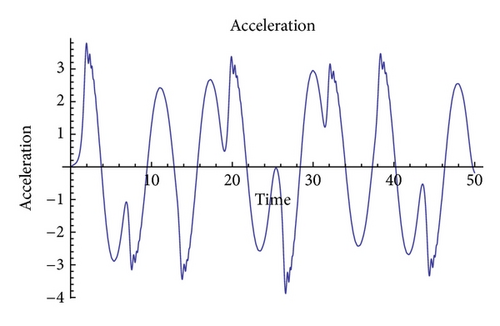
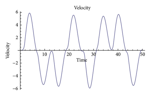
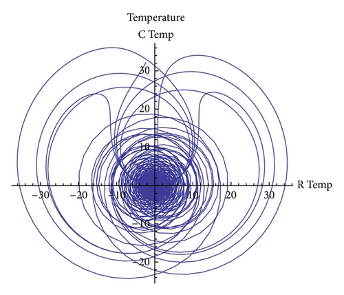
The simulations of the numerical experiments done for large values of ɛ, for instance, ɛ ranging from 2 to 1000, show that the system exhibits a pattern of chaotic behavior. For relatively large values of viscoelastic components, chaotic behaviors are observed. For all the values of heat flux B, starting from 1 to 10000, this chaotic behavior is observed (see Table 2). To illustrate the previously stated chaotic behavior, we observe the plots obtained for the values of ɛ = 10 and B = 50.
In Figure 1, we show a time graph of acceleration for a large value of the viscoelastic parameter ɛ. The acceleration ranges from −3.5 to 3.5. Since the very beginning, it displays a chaotic behavior. The curve is not very erratic although it does not show any sort of periodicity. As velocity is the time integral of acceleration, in Figure 2, the curve does not present abrupt changes close to some maxima and minima, but the nonperiodic features are also captured by this observable.
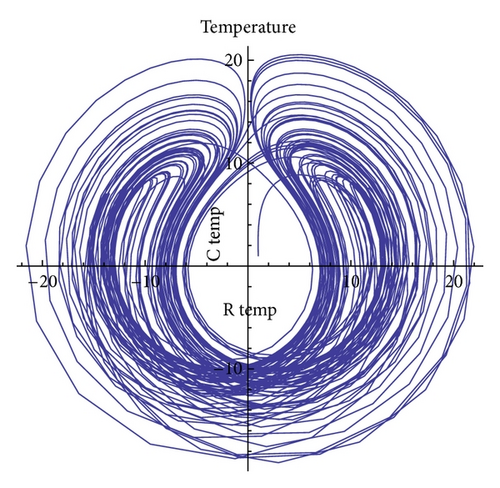
In Figure 3, we show a phase-diagram plot for the real and imaginary parts of the temperature. As expected, it also exhibits a nonperiodic pattern in which the trajectory in this phase-plane moves inwards and outwards the graph. This graph illustrates the complex underlying dynamics of the attractor (of which Figure 3 is a two-dimensional projection).
This sort of behavior remains similar for other values of B as long as the viscoelastic parameter takes larger than unity values as summarized in Table 2. In other words, the elastic effects introduce a memory effect in the dynamics which avoids the system to fully stabilize but, rather, viscoelasticity sustains the chaotic pattern. This memory effect can be understood from (3).
To sum up this section, large values of the viscoelastic parameter ɛ result on sustained chaotic behaviors. The dynamics becomes more complex, characterized in all the cases by periods of chaos and of violent oscillations, giving an idea of the complexity of the solutions of the system under these variables. In the detailed analysis of the evolution of the acceleration, velocity, and temperature, we say that the chaotic behavior of the system reveals the chaotic nature of the viscoelastic fluids.
4.1.2. Transient Irregular Behavior Followed by Stable Behavior for ɛ = 0.1 to 1
For values of ɛ ranging from 0.1 to 1, the system tends towards a stable fixed point, although it is still chaotic in the initial stages. This transient irregular behavior followed by equilibrium is shown in Figures 4, 5, and 6.
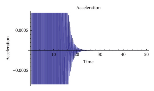
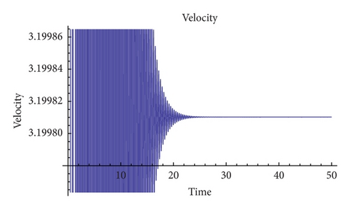
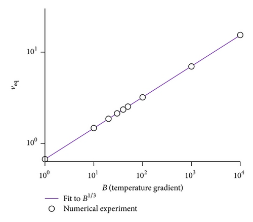
The general behavior of acceleration is that it has a chaotic outburst in the initial stages. But as time progresses it tends to stabilize, attaining equilibria. The velocity too, in the initial stages, when the time period is less than 20 units, is very inconsistent and at times unpredictable. But as the time progresses, velocity converges to a stable fixed point. Interestingly, this fixed point for the velocity is not trivial (v ≠ 0) but, on the contrary, it depends strongly on the choice of the parameters. Specifically, in Table 1, we summarize this asymptotic value. Physically, this means that the fluid inside the thermosyphon performs sustained flow in the same direction over time. This stage could be identified by the existence of convective rolls in a fully spatially extended system.
| B | ε = 1 | ε = 0.1 |
|---|---|---|
| 1 | 0.6718 | 0.6718 |
| 10 | 1.4723 | 1.4723 |
| 20 | 1.8601 | 1.8601 |
| 30 | 2.1325 | 2.1325 |
| 40 | 2.3495 | 2.3495 |
| 50 | 2.5329 | 2.5329 |
| 100 | 3.1998 | 3.1998 |
| 1000 | 6.9800 | 6.9800 |
| 10000 | 15.430 | 15.430 |
| B/ε | 10−4 | 10−3 | 10−2 | 10−1 | 100 | 101 | 102 |
|---|---|---|---|---|---|---|---|
| 1 | CS | CS | CS | CS | CS | C | C |
| 10 | CS | CS | CS | CS | CS | C | C |
| 20 | CS | CS | CS | CS | CS | C | C |
| 30 | CP | CP | CP | CS | CS | C | C |
| 40 | CP | CP | CP | CS | CS | C | C |
| 50 | CP | CP | CP | CS | CS | C | C |
| 100 | P | P | CP | CS | CS | C | C |
| 1000 | CP | CP | CP | CS | CS | C | C |
| 10000 | CP | CP | CP | CS | CS | C | C |
It is worth noting in Table 1 that both columns have the same value for the asymptotic velocity. This is a signature that viscoelastic effects do not play any role in this case (so memory effects are damped out after the early chaotic transient).
Another comment regarding Table 1 concerns the role of the parameter B. Roughly, B accounts for the scale of temperature gradients inside the thermosyphon. These results suggest that higher temperature gradients produce higher values of the sustained stationary velocity. Actually, as shown in Figure 6, the equilibrium velocity scales with B nontrivially (as a power law with exponent 1/3 approximately).
To sum up this section, we conclude that although the system has a chaotic initial transient, it tends to stabilize at longer times reaching a temperature gradient dependent equilibrium velocity. Notwithstanding, this asymptotic velocity depends nontrivially on temperature as a power law, being this a signature of the underlying nonlinearity of the equations.
4.1.3. Transition to Periodic Pattern of Behaviors for Small Values of ɛ
When the viscoelastic effects are gradually less important (values of ɛ between 0.01 and 0.0001), the system exhibits different behaviors as a function of the temperature gradient (see Table 2). For lower values of B, the system behaves in a similar fashion as for higher values of ɛ. On the contrary, for larger values of B, the system displays a periodic pattern. As in the previous case, both long-term behaviors may be preceded by an initial chaotic transient (probably caused by viscoelasticity).
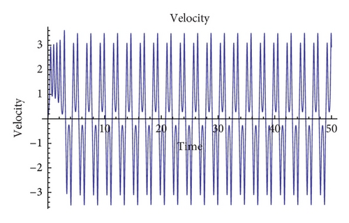
To illustrate this, in Figure 7, we show a periodic (nontrivial) behavior for ɛ = 0.001. In some cases, the initial transient cannot be distinguished from the periodic one and we refer it simply to periodic type in Table 2.
In Figure 8, we show the phase-space of the complex components of the temperature. Although at first sight it resembles a typical chaotic attractor motif, after the mentioned initial transient, the trajectories are overlapped for longer times.
Thus, in order to summarize the information covered in the last three subsections, we collect all the outcomes of the model in Table 2.
4.2. Dynamics of the Thermosyphon with Heat Diffusion (ν ≠ 0)
In this case, to avoid unnecessary repetitions in the text, we focus on the main differences between this case and that in Section 4.1.
| B/ε | 10−4 | 10−3 | 10−2 | 10−1 | 100 | 101 | 102 |
|---|---|---|---|---|---|---|---|
| 1 | CS | CS | CS | CS | CS | CS | CS |
| 10 | CS | CS | CS | CS | CS | CS | CS |
| 20 | CS | CS | CS | CS | CS | CS | CS |
| 30 | CS | CS | CS | CS | CS | CS | CS |
| 40 | P | P | P | CS | CS | CS | CS |
| 50 | P | P | P | CS | CS | CS | CS |
| 100 | P | P | P | CS | CS | CS | CS |
| 1000 | P | P | P | CS | CS | CS | CS |
| 10000 | P | P | P | CS | CS | CS | CS |
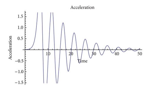
So, here we will only illustrate the most interesting behaviors with two examples. The first one takes the values of heat diffusion ν = 1, ɛ = 5, and B = 1000. As shown in Figure 9, the acceleration performs a series of damped oscillations that eventually stabilizes.
Similarly, the second example (Figure 10) takes the values ν = 2, ɛ = 5, and B = 1000. The behavior is qualitatively equal but the period of the oscillations is enlarged. In Table 3, we summarize the interaction between the tuning parameters.
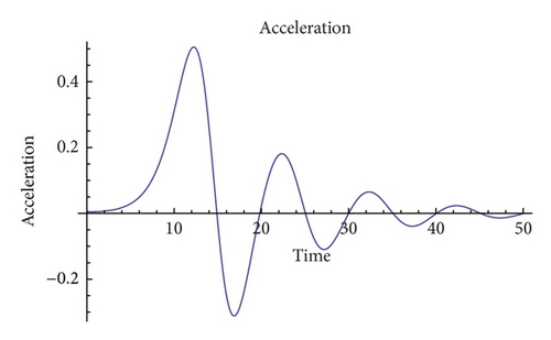
To sum up this section, we have found that greater values of the heat diffusion, ν, smoothen the dynamics of the system which, invariably, tends to stabilize, either reaching an equilibrium steady state or stable periodic orbits. These two behaviors are governed by the value of the temperature gradient which in a similar fashion as in Section 4.1 tends to produce richer behaviors for large values.
5. Conclusion
In this work, we have derived a novel system of equations to study the behavior of a viscoelastic material inside a thermosyphon. This model serves as a preliminary simplification of a more complex fully spatially extend system. This model illustrates the presence/absence of complex chaotic behaviors and also enables to relate them with the underlying viscoelastic (memory effects).
The main result is that we are able to prove that the original system (which involves both ordinary and partial different equations) possesses an inertial manifold in which the dynamics can be accurately described by a system of ODEs. By numerical integration of the reduced equations, we have been able to better understand the role of viscoelasticity (as opposed to a simpler Newtonian fluid) through the parameter ɛ. This parameter is a nondimensional version of the so-called Maxwellian viscoelastic time [4] which accounts for memory effects.
Our results suggest that in the absence of heat diffusion (ν = 0), a large value of ɛ drives the dynamics to chaotic behaviors for all the physical observable (acceleration, velocity, and temperature). As the value of ɛ gradually decreases, the system is no longer chaotic but stable or periodic. Notably, these results cannot be understood in terms of a boundary layer theory as the attractor of the dynamics changes dramatically when the second-order derivative term ɛd2v/dt2 is introduced in (5).
Physically, this induction of chaotic behaviors can be rationalized in terms of the memory effects inherent to viscoelastic models explicitly shown in (3). Thus, in the same way as delayed equations are known to produce chaos, even in the simplest situations, viscoelasticity apparently produces the same kind of transition (see, e.g., [25]).
Other interesting results are related to the effect of heat diffusion. We have found that as the heat diffusion is not zero, the system tends to stabilize either to a fixed equilibrium point or to a (ν-dependent periodicity) periodic orbit. This abrupt change in the qualitative behavior of the system is, again, due to the fact that the term νd2T/dx2 is a singular perturbation that changes the type of equation for the temperature from hyperbolic to parabolic, which justifies the explicit analysis of each situation separately in Section 2.
Our work can be generalized in many different ways, from changing the constitutive equation (from Maxwellian to other more complex situations) or to include shear-thinning effects [4] common to many non-Newtonian materials. Shear thinning is the manifestation of a shear-rate-dependent viscosity. Thus, it is commonly observed that many fluids reduce their resistance to flow for large enough imposed stresses (in our case, temperature gradients), for instance, tooth paste, paint, or lava. In principle, shear thinning means that the viscosity is smaller for higher velocities what could help to sustain oscillations once they have been formed inside the loop. However, as shown in the present work, this sort of hand waving analysis might lead to erroneous conclusions, and a detailed consideration of those effects deserves further (and deeper) investigation. These generalizations will be the aim of future works.
Acknowledgments
This work is partially supported by projects MTM2009-07540, GR58/08 Grupo 920894 BSCH-UCM, Grupo de Investigación CADEDIF, and FIS2009-12964-C05-03, Spain, and partially supported by Grant MTM2012-31298 from Ministerio de Economia y Competitividad, Spain.
Appendix
Boundary Layer Theory
The system of (5) can be seen as a singular perturbation problem provided that when ɛ = 0, the order of the differential equation reduces to one. In order to provide some insight about the solutions of those equations, a standard boundary layer theory is customary (see, e.g., [26]).
Besides, the outer problem is defined as the naive approximation ɛ → 0. Thus, the system of (5) reduces to that in [11] with an effective initial condition given by vmatching. So one would expect the same qualitative behaviors as in that work.
For instance, if the parameter B = 10, the model in [11] predicts a stable behavior. However, as shown in Table 2 (second row), increasing the value of ɛ induces a chaotic behavior. Naturally, different values of the parameters (including B) would provide different values of ɛ for which the trivial case ɛ → 0 cannot account for the observed dynamics (even for small enough values of ɛ).
This simple analysis shows the intrinsic complexity of the physical problem when viscoelasticity is considered and, more importantly, the need to study every parameter set in detail to provide an accurate description of the type of dynamics in which the system evolves.


