The previous efforts toward single period inventory problem with price-dependent demand only investigate the optimal order quantity to minimize the total inventory costs; however, there is no method in the literature to avoid unwanted costs due to the deviation between the actual demand and the previously estimated demand. To fill this gap, the present paper supposes that stochastic demand rate with normal distribution is sensitive to the selling price; this means that increasing the selling price would decrease the demand rate and vice versa. After monitoring the consumption trend within a section of the period, a new selling price is implemented to change the demand rate and reduce the shortage or salvage costs at the end of the period. Three functions were suggested to represent the demand rate as a function of selling price, and the numerical analysis was implemented to solve the proposed problem. Finally, an illustrative numerical example was solved for different configurations in order to show the advantages of the proposed model. The results revealed that there is a significant improvement in the system costs when price revision is considered.

1. Introduction

Inventory management is an important task in the business operations. The classical single period problem (SPP) deals with the purchasing inventory problem for single-period products, such as perishable or seasonal goods. The SPP has been popularly researched in the last decade, because of its extensive application in the inventory management of the products with short life cycles (e.g., fashion clothes and electronic products [1]). The authors made extensions to incorporate real world situations in SPP (for further information refer to Khouja [2]); however, there are two important problems in SPP; the first one is how to be in front of demand’s uncertainty in the real dynamic global condition and the other one is how to deal with the demand pattern which is dependent to the selling price.

For the price-dependent demand background, Whitin [3] assumed that the expected demand is a function of price, and by using incremental analysis, he derived the necessary optimality condition. Whitin then provided closed-form expressions for the optimal price, which is used to find the optimal order quantity for a demand with a rectangular distribution. Mills [4] assumed demand to be a random variable with an expected value that is decreasing in price and with constant variance. Mills derived the necessary optimality conditions and provided further analysis for the case of demand with rectangular distribution. Karlin and Carr [5] replaced the additive relation presented by Mills [4] with the multiplicative relation for the price-dependent demand where the expected price is an exponential function of two positive constants with the additional restriction that random variable obeys a cumulative distribution function with a mean of 1. A. H. L. Lau and H. S. Lau [6] developed a price-dependent demand model, in which the demand’s mean, standard deviation, skewness, and kurtosis are all functions of price. The proposed model was constructed based on the method of moments, which equates the moments of the distribution to their empirical averages in the data. Polatoglu [7] considered the simultaneous pricing and procurement decisions. Three kinds of models (including additive, multiplicative, and riskless models) were used to represent the random demand as a function of selling price. Polatoglu analyzed the SPP under general demand uncertainty to reveal the fundamental properties of the model independent of the demand pattern. Polatoglu and Sahin [8] studied a periodic inventory model with stochastic demand, which is dependent on the unit price. Abad and Jaggi [9] considered the problem of setting unit price and length of the credit period with price sensitive demand. A. H. L. Lau and H. S. Lau [10] studied the effect of five different price-dependent deterministic demand functions and showed that sometimes a slightly different demand function can lead to large change in the optimal solutions of the model. Banerjee and Sharma [11] considered a deterministic inventory model for a commodity with seasonal demand. In this model, the product under consideration has general price- and time-dependent seasonal demand rate. Simultaneous decisions were taken regarding the number of seasonal intervals before replenishment, the optimal order quantity, and the selling price, so as to maximize the net profit per unit time.

From the other side, to overcome the problem of difference between the real demand and estimated demand, that causes overstock or understock at the end of period, Bitran and Mondschein [12] characterized the optimal pricing policies as functions of time and inventory to present a continuous time model where the seller faces a stochastic arrival of customers with different valuations of the product. They showed that the optimal pricing policy is to successively discount the product during the season and promote a liquidation sale at the end of the planning horizon. Khouja [13] extended the SPP to the case in which demand is price dependent. Multiple discounts with prices under the control of the newsvendor were used to sell excess inventory. Two algorithms were developed to determine the optimal number of discounts under fixed discounting cost for a given order quantity and realization of demand. Also, the joint determination of the order quantity and initial price was analyzed. Şen and Zhang [14] considered the newsboy model with multiple demand classes, each with a different selling price. Optimal order quantity and demand values in each of the demand classes were determined by following a policy based on protecting the sales in the higher fare class and limiting the sales in the lower fare class. Feng and Xiao [15] investigated optimal times to switch between prices based on the remaining season and inventory; it was assumed that demand is price dependent with Poisson process. Petruzzi and Dada [16] presented a multiperiod newsvendor model to determine optimal stocking and pricing policies over time when a given market parameter of the demand process, though fixed, but initially is unknown. Chung et al. [17] extended the classical SPP by allowing the retailer to make an in-season price adjustment after conducting a review and using the realized demand to obtain an accurate estimate of the remaining demand. In order to obtain optimal order quantity and adjusted price after the review time, they considered a zero salvage value, small variance after review time, deterministic function of price, and information before review time.

It is noticeable that pricing policies and price-dependent demand models have extensive applications in the other inventory fields; for instance, You and Chen [18] attempted to explore the inventory replenishment policy in EOQ setting by assuming that demand is sensitive to stock and selling price. In the proposed approach, optimal decision rules were surveyed without price change, with a single price change, and with two price changes. Also In the extension of this paper, Mo et al. [19] analyzed the optimal decisions for general value of n changes. Sinha and Sarmah [20] developed a single-vendor multibuyer discount pricing model under stochastic demand information. In this model, the vendor offers multiple pricing schedules to encourage the buyers to adopt the global optimal policy instead of their individual optimal ordering policy. Chen et al. [21] studied a coordination contract for a supplier-retailer channel with stochastic price-dependent demand. They supposed a two-stage optimization problem where in the first stage the supplier decides the amount of capacity reservation, and in the second stage after updating demand information, the retailer determines the order quantity and the retail price. Also, Chiu et al. [22] presented a policy for channel coordination in supply chains with both additive and multiplicative price-dependent demands. The proposed policy combines the use of wholesale price, channel rebate, and returns.

The previous efforts toward single period inventory problem with price-dependent demand only investigate the optimal order quantity to minimize the total inventory costs; however, there is no method in the literature to avoid unwanted costs due to the deviation between the actual demand and previously estimated demand. To fill this gap, the present paper supposes that, the stochastic demand rate with normal distribution is sensitive to the selling price; this means that increasing the selling price would decrease the demand rate (by affecting mean and variance of the demand rate distribution) and vice versa. After monitoring the consumption trend within a section of the period, a new selling price is implemented to change the demand rate and reduce the shortage or salvage costs at the end of the period. Three functions are suggested to represent the demand rate as a function of selling price, and numerical analysis is implemented to solve the proposed problem. Finally, a numerical example is solved for various configurations, and sensitivity analysis is performed to show the efficiency of the proposed approach.

2. The Classical Newsvendor Model

Single period problem or newsvendor problem is one of the most well-known inventory models which attempts to find order quantity within stochastic demand in a single period so as to maximize the expected profit or minimize the expected costs (these terms are equal). The assumptions of this model are as follows.

(i)
Demand is a stochastic variable.
(ii)
Unsold items are sold by a discount (salvaged) or disposed at the end of the period.
(iii)
Shortage is allowed.
(iv)
Only one purchase order is allowed and the ordered lot is placed at the beginning of the period.

For the classical newsvendor problem, the optimum order quantity (Q^*) can be easily obtained through the following equation [2]:

()

where p is the unit selling price, c is the unit procurement cost, v is the unit salvage value, s is the unit shortage cost, and F⁻¹(·) denotes the inverse of the cumulative distribution function of demand.

3. The Newsvendor Model with Inventory Revision

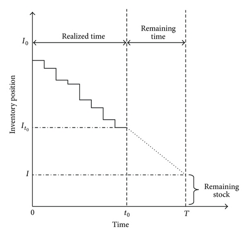
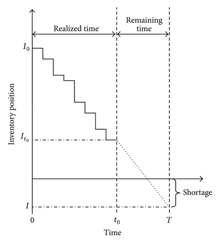
The previous efforts toward single period problem with price-dependent demand only investigate the optimal order quantity to minimize the total inventory costs; however, there is no method in the literature to avoid unwanted costs due to the deviation between the actual demand and previously estimated demand. To fill this gap, the present paper supposes that demand rate is sensitive to the selling price; this means that increasing the selling price would decrease the demand rate and vice versa. After monitoring the consumption trend within a section of the period, a new selling price is implemented to change the demand rate and reduce the shortage or salvage costs at the end of the period. For illustration, in Figure 1, demand rate within the interval [0, t₀] shows that it is most likely to have some remaining stock at the end of the period; hence, we should decrease the selling price to increase the demand rate and consequently avoid the salvage cost. From the other side, in Figure 2, demand rate within the interval [0, t₀] shows that it is most likely to have some unsatisfied demand at the end of the period, and therefore we should increase the selling price in order to decrease demand rate and consequently reduce the shortage cost.

Details are in the caption following the image — **Figure 1**
Open in figure viewer PowerPoint

Consumption trend and predicted remaining stock at the end of the period.

The assumptions in this work are as follows.

(i)
The demand rate is a stochastic normal variable.
(ii)
The parameters of the demand rate distribution are unknown before the beginning of the period.
(iii)
The demand rate is sensitive to the selling price.
(iv)
Mean and variance of the demand rate are a deterministic functions of the selling price.
(v)
The changed demand rate is stable after price revision.
(vi)
The order quantity is known and placed at the beginning of the period as the initial inventory level.

Note that, since the parameters of the demand rate distribution are unknown before the beginning of the period, we can use the expert’s opinion to obtain initial inventory level, or the information of the similar commodities can be used to obtain it by using (1).

Also, the following notations are used in the mathematical model.

I₀: initial inventory level at the beginning of the period.
t₀: revision point.
p₀: selling price before price revision.
p: unit selling price after price revision.
c: unit procurement cost.
c₀: unit salvage (or dispose) value.
s: unit shortage cost.
D: stochastic demand rate after price revision, where .
R_p: variation ratio in the demand rate when revising selling price.
: optimum revised price based on the actual demand rate distribution.
: optimum revised price based on the estimated demand rate within the interval [0, t₀].
NPV_A: optimum net present value based on the actual demand rate distribution.
NPV_E: optimum net present value based on the estimated demand rate.

As it was mentioned, the parameters of the demand rate distribution are unknown at the zero time. These parameters can be estimated based on the consumption trend. So

and

are introduced as the mean and variance of demand rate before the revision point (t₀), respectively. These parameters are estimated as follows:

()

In (2), t₀ should be as large enough to appropriately estimate

and

; however, if we take t₀ too large, less time remains to adjust the inventory level. Therefore, we need to establish a compromise between the remaining time and the use of the past information. For commodities, which have a selling period more than 30 days, using the information of 10–15 days may be sufficient to estimate the parameters of the demand rate distribution.

Now, in order to represent the demand rate after revision point (D) in terms of selling price p, we assume that

, where μ_D and

are the mean and variance of demand rate distribution after revision point, respectively. Since D is directly proportional to R_p, μ_D and

are estimated as follows:

()

In (3), R_p is inversely proportional to p, that is, increasing p would decrease R_p and consequently decrease D, and vice versa. Therefore, D is sensitive to p.

To represent the inverse relation between p and R_p, we present several ratio functions that satisfy the following requirements:

(i)
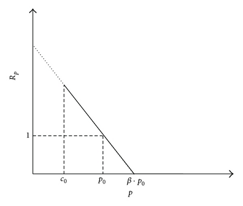
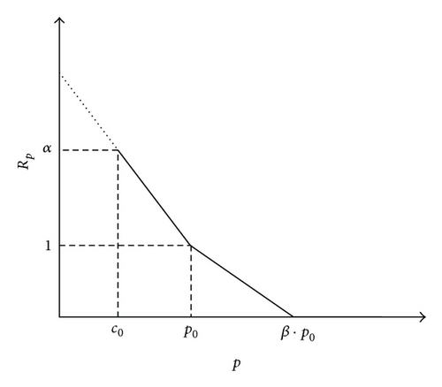
R_p = 1, for all p = p₀.
(ii)
∂R_p/∂p ≤ 0.
(iii)
lim_p→∞R_p = 0.
(iv)
R_p = 1, for all p = p₀.

Then, the first requirement indicates that the demand rate would not change if the selling price is the same before being offered, the second one represents that R_p and p have inverse relation, the third one implies that the demand rate would become almost zero if the selling price increases significantly, and the last one represents that demand rate at any moment is a positive value. It is necessary to note that the revised price should be greater than c₀, because we are sure that the remaining stock can be sold without any trouble.

3.1. Linear Ratio Function

In the linear ratio function, it is assumed that the relation between R_p and p is approximately linear (see Figure 3); therefore, the following function can be implemented to represent it.

()

In (4), β is the price elasticity; the higher the β, the more elasticity there is.

3.2. Two-Segment Ratio Function

Since the linear ratio function is not more flexible, we present the two-segment ratio function. This function consists of two linear sections (see Figure 4). The inverse relation between R_p and p for the two-segment ratio function can be expressed as follows:

()

In (5), α is the variation ratio in the demand rate, when it is assumed that p = c₀, and β is the price elasticity.

3.3. Exponential Ratio Function

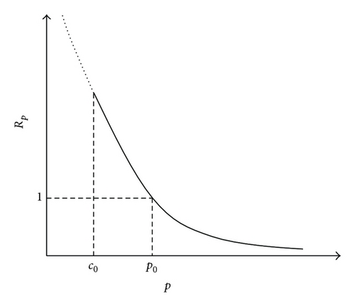
Another flexible function which corresponds to the inverse relation between p and R_p is the exponential ratio function (see Figure 5). This function can be expressed as follows:

()

Various values for α and β in (6) can yield different ration functions.

The presented parameters in each ratio function, that is, α and β, can be obtained according to the expert’s opinion or using statistical methods such as regression.

After selecting an appropriate ratio function for the problem, in the next step, in order to evaluate the net present value (NPV), we should specify the probability distribution of the inventory position (I) at the end of the period. As D is distributed normally, that is,

, and since

, I is also distributed normally with parameters μ_I and

, that is,

, where

()

After specifying the distribution of I, we write NPV based on I to analyze optimum value of selling price.

()

In (8), if I ≥ 0, then we have salvage cost; otherwise, we have shortage cost.

Now, we define μ_NPV as the expected value of NPV and obtain it as follows:

()

After simplifying (9), we have

()

where ϕ(·) is the cumulative distribution function of the standard normal distribution.

As it is obvious in (10), the term of is dependent on p and can only be numerically obtained; hence, we cannot solve dμ_NPV/dp = 0 to obtain the optimum revised price (p^*). Therefore, we implement the numerical analysis to obtain p^*. The pseudocodes of the proposed numerical analysis have been included in Pseudocodes 1 and 2.

Pseudocode 1: Pseudocode for obtaining the best revised price within the interval (a, b).

Function p(a, b)
ε ← 〈〉 ⊳ Initialize ε; where ε is the length of each step at each iteration
Δ ← 〈〉 ⊳ Initialize Δ; Δ > 2ε where Δ is the calculation accuracy
p₁ = a
p₂ = b
repeat
p = (p₁ + p₂)/2
if μ_NPV(p) > μ_NPV(p + ε) then
p₂ = p
else
p₁ = p
End if
until p₂ − p₁ < Δ ⊳ Check finishing criterion
return p
End Function

Pseudocode 2: Pseudocode for obtaining the optimal revised price (p^*).

Function p^*
case ratio_function of
Linear:
p^* = p(c₀, βp₀)
Two_Segment:
p₁ = p(c₀, p₀)
p₂ = p(c₀, βp₀)
if μ_NPV(p₁) > μ_NPV(p₂) then
p^* = p₁
else
p^* = p₂
End if
Exponential:
p^* = p(c₀, ∞)
End case
return p^*
End Function

4. An Illustrative Example

In this section, an illustrative numerical example has been included to show the efficiency of the proposed approach. The results of the proposed model (with price revision) are compared against that without price revision. The consumption trend for the first 15 days has been generated randomly according to the normal distribution with μ = 18, σ² = 25 and included in Table 1. The other parameters are assumed as follows: c = 50, c₀ = 20, s = 30, p₀ = 80, T = 30, and t₀ = 15.

Table 1. Consumption trend for the first 15 days.

Day	1	2	3	4	5	6	7	8	9	10	11	12	13	14	15
Demand	16	12	19	24	24	27	7	17	23	13	15	10	9	13	14

Table 2 shows the expected profit without price revision. This example is investigated for the three types of ratio functions and three levels of the initial inventory (I₀), including 400, 500, and 600, and the results are summarized in Tables 3, 4, and 5, respectively. In these tables, the columns of and indicate the optimum solutions based on the estimated demand rate within the interval [0, t₀] (i.e., the proposed approach), the columns of and show the optimum solutions based on the actual demand rate, with the mean 18 and variance 25 (which are unknown for us), the column of shows the expected NPV based on the actual demand rate for , and finally the last column shows the relative gap between and expected NPV without the price revision included in the last row of Table 2 (i.e., NPV_W); this column has been calculated as follows: . Also, Figures 6, 7, and 8 display the plots of NPV_E and NPV_A against p for three sample cases. In these figures, the terms of “actual” and “estimated” refer to NPV_A and NPV_E, respectively.

Table 2. Computational result without price revision.

Primary inventory (I₀)	400	500	600
Expected NPV without price revision (NPV_W)	1320.0	7058.4	5490.0

Table 3. Computational results considering I₀ = 400.

Ratio function	α	β						Imp. (%)
Linear	—	2	110.6	8529	114.5	9442	9061	586.4%
	—	1.8	103.9	7633	107.3	8404	7986	505.0%
	—	1.5	94.4	6311	96.8	6859	6439	387.8%

Two-segment	6	2	110.6	8529	114.5	9442	9061	586.4%
	5	1.8	103.9	7633	107.3	8404	7986	505.0%
	7	1.4	91.4	5877	93.4	6348	5935	349.6%

Exponential	1.2	1.9	92.1	5928	94.8	6516	6096	361.8%
	1.7	2.1	89.6	5594	91.8	6101	5674	329.9%
	1.2	0.8	100.8	7067	104.9	7933	7533	470.7%
	0	2	99.2	6865	102.7	7646	7267	450.6%

Table 4. Computational results considering I₀ = 500.

Ratio function	α	β						Imp. (%)
Linear	—	2	90.7	7165	92.3	8782	8761	24.1%
	—	1.8	85.3	6795	87.9	8267	8137	15.3%
	—	1.5	80.7	6528	83.5	7657	7275	3.1%

Two-segment	6	2	90.7	7165	92.3	8782	8761	24.1%
	5	1.8	85.3	6795	87.9	8267	8137	15.3%
	7	1.4	79.4	6678	82.4	7496	6628	−6.1%

Exponential	1.2	1.9	79.5	6530	81.9	7404	6852	−2.9%
	1.7	2.1	79.2	6557	81.4	7323	6691	−5.2%
	1.2	0.8	80.8	6530	84.1	7715	7301	3.4%
	0	2	80.8	6530	83.8	7700	7301	3.4%

Table 5. Computational results considering I₀ = 600.

Ratio function	α	β						Imp. (%)
Linear	—	2	89.9	4174	89.9	5827	5827	6.1%
	—	1.8	81.9	3885	81.9	5507	5507	0.3%
	—	1.5	71.0	4455	72.5	6077	6027	9.8%

Two-segment	6	2	74.7	7572	76.1	8450	7726	40.7%
	5	1.8	73.6	7134	75.4	8142	7362	34.1%
	7	1.4	75.4	7873	76.8	8675	7874	43.4%

Exponential	1.2	1.9	71.5	6294	73.7	7423	6791	23.7%
	1.7	2.1	72.6	6824	74.6	7822	7037	28.2%
	1.2	0.8	68.8	4978	71.8	6404	5930	8.0%
	0	2	69.1	4831	71.8	6319	5985	9.0%

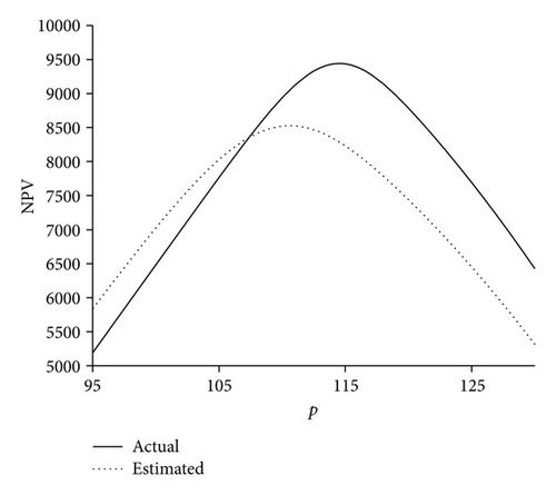
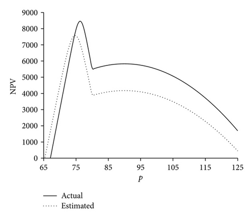
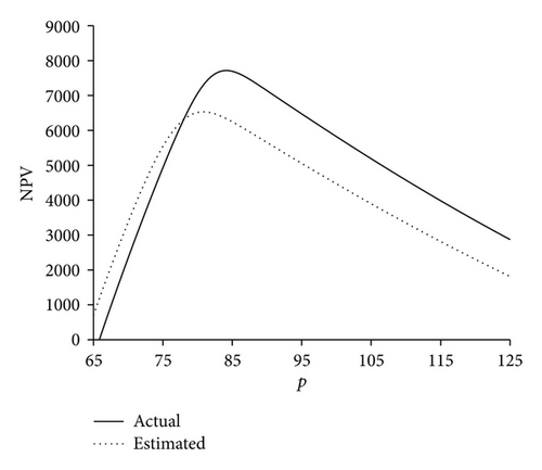
The computational results indicated that in all the cases, except three cases in Table 4, the proposed approach gives better results in comparison with the state in which price revision is not considered. Also, for those cases in which the improvement percent is negative, the amount of loss in the expected NPV is insignificant. It can be observed that the optimum revised price for the estimated demand rate () has no significant difference with that for the actual demand rate (); this implies that monitoring demand rate within the interval [0, t₀] to estimate demand rate can provide an efficient approximation for the problem.

5. Sensitivity Analysis

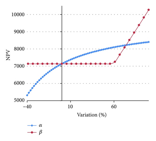
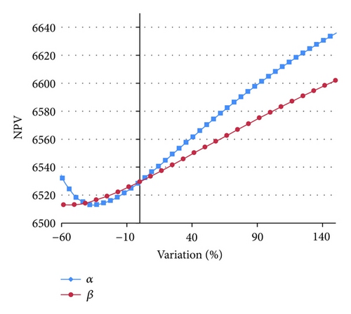
In this section, we investigate the model’s sensitivity with respect to the different parameters of the ratio functions. The relationship between NPV_E and different values of α and β, for the two-segment and exponential ratio functions, have been plotted in Figures 9 and 10, respectively. From Figures 9 and 10, we can observe that the two-segment ratio function is more sensitive than the exponential ratio function. In the two-segment ratio function, α is more sensitive than β within the interval [−40,60); conversely, within the interval [60, ∞), β is more sensitive than α. Also in the exponential ratio function, α is generally more sensitive than β.

6. Conclusion and Directions for Future Research

In this paper, we presented a price-dependent model for the single period inventory problem. Considering the fact that the distribution of the demand rate is unknown at the beginning of the period, we attempted to estimate the parameters of the demand rate distribution by investigating the consumption trend within a specific section of the period. Three functions were suggested to represent the demand rate as a function of selling price. We attempted to find the optimum revised price so as to maximize the expected NPV at the end of the period. A numerical example was solved for different configurations, and the results were compared against the state in which price revision is not considered. The results revealed significant improvement when the price revision is considered. Furthermore, it was concluded that the optimum revised price for the estimated demand rate has no significant difference with that for the actual demand rate; this implies that monitoring the consumption trend within a section of the period to estimate the parameters of the demand rate distribution can provide an efficient approximation for the problem.

At the end, for the future researches, we suggest the following guidelines.

(i)
Developing the proposed approach for dynamic price revision.
(ii)
Using the other functions to represent the demand rate as a function of selling price, such as multisegment, combinational, and fuzzy functions.
(iii)
Developing a mathematical method in order to obtain revision point with more accuracy.
(iv)
Considering time-dependent holding cost in the model.
(v)
Using other distribution functions such as uniform distribution and Poisson distribution, as the distribution of the demand rate.

These suggestions remain critical issues for the future studies.

References

1 Zhang J. L., Lee C. Y., and Chen J., Inventory control problem with freight cost and stochastic demand, Operations Research Letters. (2009) 37, no. 6, 443–446, 2-s2.0-70349814404, https://doi.org/10.1016/j.orl.2009.04.009.
Web of Science® Google Scholar
2 Khouja M., The single-period (news-vendor) problem: literature review and suggestions for future research, Omega. (1999) 27, no. 5, 537–553, 2-s2.0-0001552617, https://doi.org/10.1016/S0305-0483(99)00017-1.
Google Scholar
3 Whitin T. M., Inventory control and price theory, Management Science. (1955) 2, 61–68.
Google Scholar
4 Mills E. S., Uncertainty and price theory, The Quarterly Journal of Economics. (1959) 73, 116–130.
Google Scholar
5 Karlin S. and Carr C. R., K. J. Arrow and H. Scarf, Prices and optimal inventory policy, Studies in Applied Probability and Management Science, 1962, Stanford University Press, Stanford, Calif, USA, 159–172.
Google Scholar
6 Lau A. H. L. and Lau H. S., The newsboy problem with price-dependent demand distribution, IIE Transactions. (1988) 20, no. 2, 168–175, 2-s2.0-0024031728.
Google Scholar
7 Polatoglu L. H., Optimal order quantity and pricing decisions in single-period inventory systems, International Journal of Production Economics. (1991) 23, no. 1–3, 175–185, 2-s2.0-0026244549.
Google Scholar
8 Polatoglu H. and Sahin I., Optimal procurement policies under price-dependent demand, International Journal of Production Economics. (2000) 65, no. 2, 141–171, 2-s2.0-0033876387, https://doi.org/10.1016/S0925-5273(98)00240-0.
Google Scholar
9 Abad P. L. and Jaggi C. K., A joint approach for setting unit price and the length of the credit period for a seller when end demand is price sensitive, International Journal of Production Economics. (2003) 183, 115–122.
Google Scholar
10 Lau A. H. L. and Lau H. S., Effects of a demand-curve′s shape on the optimal solutions of a multi-echelon inventory/pricing model, European Journal of Operational Research. (2003) 147, no. 3, 530–548, 2-s2.0-0037449228, https://doi.org/10.1016/S0377-2217(02)00291-6.
Google Scholar
11 Banerjee S. and Sharma A., Optimal procurement and pricing policies for inventory models with price and time dependent seasonal demand, Mathematical and Computer Modelling. (2010) 51, no. 5-6, 700–714, 2-s2.0-74149092697, https://doi.org/10.1016/j.mcm.2009.10.022.
Google Scholar
12 Bitran G. R. and Mondschein S. V., Periodic pricing of seasonal products in retailing, Management Science. (1997) 43, no. 1, 64–79, 2-s2.0-0030622777.
Web of Science® Google Scholar
13 Khouja M. J., Optimal ordering, discounting, and pricing in the single-period problem, International Journal of Production Economics. (2000) 65, no. 2, 201–216, 2-s2.0-0033899107, https://doi.org/10.1016/S0925-5273(99)00027-4.
Google Scholar
14 Şen A. and Zhang A. X., The newsboy problem with multiple demand classes, IIE Transactions. (1999) 31, no. 5, 431–444, 2-s2.0-0032649938.
Google Scholar
15 Feng Y. and Xiao B., Optimal policies of yield management with multiple predetermined prices, Operations Research. (2000) 48, no. 2, 332–343, 2-s2.0-0034156186.
Google Scholar
16 Petruzzi N. C. and Dada M., Dynamic pricing and inventory control with learning, Naval Research Logistics. (2002) 49, no. 3, 303–325, 2-s2.0-0036533756, https://doi.org/10.1002/nav.10013.
Google Scholar
17 Chung C. S., Flynn J., and Zhu J., The newsvendor problem with an in-season price adjustment, European Journal of Operational Research. (2009) 198, no. 1, 148–156, 2-s2.0-62549122093, https://doi.org/10.1016/j.ejor.2007.10.067.
Google Scholar
18 You P. S. and Chen T. C., Dynamic pricing of seasonal goods with spot and forward purchase demands, Computers and Mathematics with Applications. (2007) 54, no. 4, 490–498, 2-s2.0-34250870799, https://doi.org/10.1016/j.camwa.2007.01.026.
Google Scholar
19 Mo J., Mi F., Zhou F., and Pan H., A note on an EOQ model with stock and price sensitive demand, Mathematical and Computer Modelling. (2009) 49, no. 9-10, 2029–2036, 2-s2.0-63449086553, https://doi.org/10.1016/j.mcm.2008.10.012.
Google Scholar
20 Sinha S. and Sarmah S. P., Single-vendor multi-buyer discount pricing model under stochastic demand environment, Computers and Industrial Engineering. (2010) 59, 945–953, https://doi.org/10.1016/j.cie.2010.09.005.
Google Scholar
21 Chen H., Chen Y., Chiu C. H., Choi T. M., and Sethi S., Coordination mechanism for the supply chain with leadtime consideration and price-dependent demand, European Journal of Operational Research. (2010) 203, no. 1, 70–80, 2-s2.0-70350776675, https://doi.org/10.1016/j.ejor.2009.07.002.
Google Scholar
22 Chiu C. H., Choi T. M., and Tang C. S., Price, rebate, and returns supply contracts for coordinating supply chains with price-dependent demands, Production and Operations Management. (2011) 20, no. 1, 81–91, 2-s2.0-79951970146, https://doi.org/10.1111/j.1937-5956.2010.01159.x.
Web of Science® Google Scholar

Citing Literature

All articles

A Price-Dependent Demand Model in the Single Period Inventory System with Price Adjustment

Abstract

1. Introduction

2. The Classical Newsvendor Model