A Start-Up Demonstration Test Involving Distant Failures
Abstract
A new procedure for determining the acceptance or rejection of a system that undergoes a start-up demonstration set of tests is presented. It is a generalization of the recently introduced CSDF model (consecutive successes distant failures). According to the new total successes consecutive successes total failures distant failures (TSCSTFDF) procedure, a unit is accepted when either a total number of successful tests or a specified number of consecutive successes are observed before a total number of failures or the occurrence of near failures which are too close to each other. The practical advantage of this new procedure is the significant reduction in the expected number of required tests together with improved second-order statistics (standard deviation).
1. Introduction
Start-up demonstration tests are performed in order to prove the reliability of power generating equipment like lawn mowers, water pumps, car batteries, and many sorts of electronic equipment. An example for an application has been mentioned by Antzoulakos et al. [1] regarding a conference center that wishes to replace its old slide projectors with modern ones. The outcomes of a set of demonstration tests that are carried out on the new projectors are recorded. The requirement may be in form of observing consecutive successes before the occurrence of a certain number of failures or before meeting a consecutive set of failures. As a result, the reliability of the equipment is determined.
Various procedures exist for deciding whether the set of tests is successful which imply the decision on accepting or rejecting the unit in question.
They are based on the commonly known theory of consecutive k-out-of-n systems [2]. Among others, there exist the consecutive successes (CS), total successes consecutive successes (TSCS), consecutive failures total failures (CSTF), consecutive successes distant failures (CSDF), and a general TSCSTFCF procedure. According to the simplest CS procedure, the equipment is accepted if there exists a certain run of successes of prespecified length (kcs) when performing the set of tests [3, 4]. The combination of the requirement for consecutive successes and/or the total number of successes (TSCS) (ks, kcs) as a basis for accepting the unit has been presented by Gera [5]. A more advanced procedure (CSTF) has been given by Balakrishnan and Chan [6], Smith and Griffith [7, 8], and Martin [9, 10]. Like before, the unit is accepted if there exists a run of successes (kcs). However, it is rejected if a certain number of failures is reached before that run (kf). More general models are the TSCSTF and TSCSTFCF procedures which have been presented by Gera [11, 12]. According to the TSCSTFCF model, a unit is accepted if either a run of successes or a total number of successes are observed before either a total number of failure or a run of failures (ks, kcs, kf, and kcf), and vice versa for rejection. The CSDF model has been recently introduced by Antzoulakos et al. [1] according to which a unit is accepted if a run of kcs consecutive successes is obtained before the occurrence of two failures that are not sufficiently distant (r) from each other. It is rejected if two failures that are not sufficiently distant from each other are met before a certain run of successes (kcs, r).
A generalization of the previously mentioned CSDF procedure is presented here: total successes consecutive successes total failures distant failures (TSCSTFDF). It involves the addition of two parameters: total number of successes (ks) and total number of failures (kf). Thus, the tested equipment is accepted if there exists a run of successes of a fixed length (kcs) or a total number of successes (ks) before either a total number of kf failures or the occurrence of two failures that have less than r − 1 successes between them (so that they are too close to each other). The following questions will be answered. What is the probability of accepting a unit undergoing such a process? What are the chances of observing a set of kcs consecutive successes before the occurrence of a set of consecutive kcf failures? Given the various parameters like kcs, ks, kf, and r, what is the expected number of tests till arriving a decision? From analysis to design, a method of determining the values of those parameters due to some optimization criterion will be presented.
The statistical properties of the new model are examined. s-independence between the tests is assumed and the probability of success of each trial (p) is assumed to be identical (i.i.d.). A practical problem is the number of required tests which surely should be as low as possible subject to some limits on the confidence level of the tests. This problem of minimizing the expected number of tests that are required is set up in form of a constrained optimization problem. It will be observed that a significant reduction in that number is achieved by using the new procedure.
The problem of estimating the underlying probability of success of each test (p) is also tackled. Previous work in this direction has been carried out by Viveros and Balakrishnan [4], Smith and Griffith [7], Gera [12], and Antzoulakos et al. [1]. Maximum likelihood (MLE) is applied to obtain interval estimation. An illustrative example is presented.
2. The TSCSTFDF Procedure
Let ks be the number of successes required for acceptance, let kcs be the number of consecutive successes required for acceptance, let kf be the number of failures yielding rejection, and let r − 2 be the maximal number of successes between failures causing rejection. Also, denote by Tns the number of successful startups throughout n tests, by Lns the length of the longest run of successes throughout n tests, and by Dnf the minimal spacing between any two adjacent failures throughout n tests. Xi is the outcome of the ith start-up test (=1 for success, =0 for failure). The previously known CSDF procedure made use only of the kcs and r parameters. Here we increase the number of parameters (TSCSTFDF), so that we will obtain significantly shortening of the number of tests required to reach a decision with respect to the tested equipment.
3. Constrained Optimization
The present procedure is a generalization of the previous CSDF introduced by Antzoulakos et al. and it is advantageous compared to the simpler model in reducing the expected number of tests required for the demonstration. Smith and Griffith [7, 8] have suggested a procedure for minimizing the expected number of tests through a correct choice of the kcs, kf parameters for the CSTF model. The optimization is carried out with respect to some constraints. Antzoulakos et al. [1] pointed out such an optimization regarding the CSDF model. Gera [12] applied this procedure to the more general TSCSTFCF. A similar procedure will be applied here using the TSCSTFDF model.
4. Interval Estimation of “p”
It is assumed here that the probability of success (p) of each unit is the same, and it is independent of the other trials (i.i.d.). Performing n tests on several units with prespecified values of ks, kf, kcs, and r, the number of successes (si) and of failures (fi) are observed for each unit. The number of tests performed on the i′th unit is given by ni = si + fi. Then, the total number of tests for all units will be given by summing on all of the ni.
5. Numerical Results
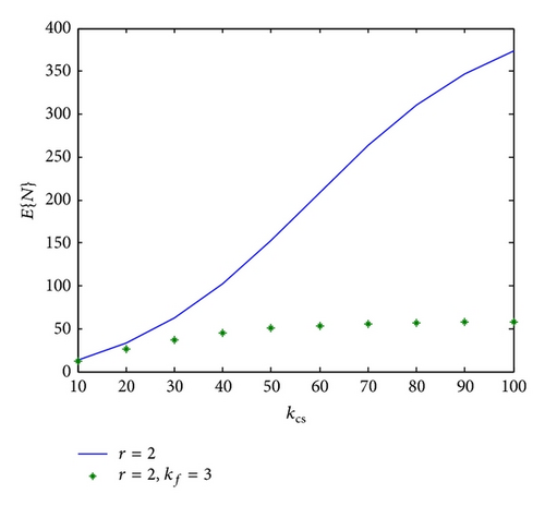
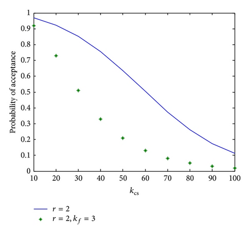
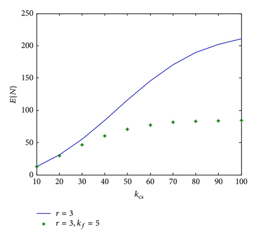
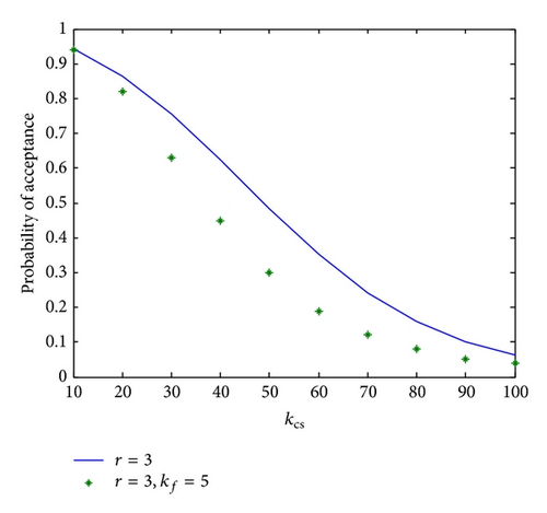
As an example, the effect of introducing additional parameters like kf on the expected number of tests and on probability of acceptance may be seen in Figures 1, 2, 3, and 4.


As to the design problem of choosing the optimal values of the parameters, they obviously depend on the values of the upper and lower probabilities and the confidence limits. The optimization procedure presented above has been applied to the test case given by Antzoulakos et al. [1]. They derived optimal values of the parameters using the simpler CSDF model. Our numerical results fully correlate theirs for that case. Using the values of pU = 0.9, pL = 0.7, α = 0.25, and β = 0.2 and applying their relation (10) for finding the expected number of tests, their results are presented in Table 1.
| kcs | r | E {N/pU} | E {N/pL} | P {a/pU} | P {a/pL} |
|---|---|---|---|---|---|
| 6 | 5 | 7.1937 | 5.8984 | 0.8159 | 0.2359 |
| 7 | 3 | 9.2897 | 7.7974 | 0.8517 | 0.2099 |
| 12 | 2 | 20.6397 | 13.6163 | 0.8124 | 0.0573 |
- pU = 0.9; pL = 0.7; α = 0.25; β = 0.2.
It is observed that the optimal values are obtained when choosing kcs = 6, r = 5 which fulfill the constraints.
We suggest an improved optimum for the same problem by using instead the more general TSCSTFDF procedure, as shown in Table 2.
| ks | kcs | kf | r | E {N/pU} | SD | P {a/pU} | P {a/pL} |
|---|---|---|---|---|---|---|---|
| 200 | 6 | 200 | 5 | 7.19 | 2.64 | 0.8159 | 0.2359 |
| 11 | 6 | 200 | 5 | 7.09 | 2.27 | 0.8210 | 0.2478 |
| 11 | 6 | 3 | 5 | 7.09 | 2.26 | 0.8185 | 0.2215 |
| 8 | 6 | 2 | 5 | 6.64 | 1.47 | 0.8046 | 0.2468 |
- The SD value is the standard deviation around E {N/pU}.
- pU = 0.9; pL = 0.7; α = 0.25; β = 0.2.
The optimal value of E{N/pU} owing to using the TSCSTFDF procedure is thus reduced significantly, 7.5% improvement, with respect to the previously derived optimum value using the CSDF model. We also gain simultaneously an enormous improvement in the value of the standard deviation. A systematic approach to locate the optimum will surely yield a further reduction in the optimal value.
The statistical inference on the value of “p” may be illustrated for instance by using the simulated data presented by Antzoulakos et al. [1] for n = 30 units by adding a value of ks = 12 to the input values of p = 0.9, kcs = 10, and r = 3. Referring to their data, the following results are shown in Table 3. The reason for terminating the set of tests is indicated in the last row (ks: reaching the limit number of successes for acceptance, kcs: encountering a run of successes for acceptance, and C0,1 and C0,2: close failures < r − 1).
| i | 1 | 2 | 3 | 4 | 5 | 6 | 7 | 8 | 9 | 10 | 11 | 12 | 13 | 14 | 15 |
| ni | 13 | 3 | 11 | 10 | 10 | 10 | 10 | 15 | 11 | 6 | 13 | 10 | 11 | 10 | 10 |
| si | 12 | 1 | 10 | 10 | 10 | 10 | 10 | 12 | 9 | 4 | 12 | 10 | 10 | 10 | 8 |
| fi | 1 | 2 | 1 | 0 | 0 | 0 | 0 | 3 | 2 | 2 | 1 | 0 | 1 | 0 | 2 |
| C | ks | C0,2 | kcs | kcs | kcs | kcs | kcs | ks | C0,2 | C0,1 | ks | kcs | kcs | kcs | C0,2 |
| i | 16 | 17 | 18 | 19 | 20 | 21 | 22 | 23 | 24 | 25 | 26 | 27 | 28 | 29 | 30 |
| ni | 15 | 5 | 14 | 13 | 12 | 11 | 13 | 10 | 6 | 13 | 12 | 13 | 4 | 13 | 13 |
| si | 11 | 3 | 12 | 12 | 11 | 10 | 12 | 10 | 4 | 12 | 11 | 12 | 2 | 12 | 12 |
| fi | 4 | 2 | 2 | 1 | 1 | 1 | 1 | 0 | 2 | 1 | 1 | 1 | 2 | 1 | 1 |
| C | C0,2 | C0,1 | ks | ks | kcs | kcs | ks | kcs | C0,2 | kcs | kcs | ks | C0,1 | ks | ks |
6. Summary and Conclusions
A new model (TSCSTFDF) has been presented for performing a set of start-up demonstration tests. It is a generalization of the previously known CSDF procedure by adding the parameters representing the total number of successes (ks) and of failures (kf) into the analysis and the design of the test procedure. The main advantage in using the more general model is in the reduction of the expected number of required tests together with improved second-order statistics. Although some more measurements need to be carried out, this advantage still seems to be significant and the procedure seems to be practical. A constrained optimization problem has been set up together with an illustrated example. Future work should involve a systematic algorithm for yielding the optimum.
Acronym
-
- CS:
-
- Total successes
-
- TSCS:
-
- Total successes consecutive successes
-
- CSTF:
-
- Consecutive successes total failures
-
- CSDF:
-
- Consecutive successes distant failures
-
- TSCSTF:
-
- Total successes consecutive successes total failures
-
- TSCSTFCF:
-
- Total successes consecutive successes total failures consecutive failures
-
- TSCSTFDF:
-
- Total successes consecutive successes total failures distant failures.
Notation
-
- p, q:
-
- Probability of success, failure of each trial
-
- ks:
-
- The number of successes required for acceptance
-
- kcs:
-
- The number of consecutive successes required for acceptance
-
- kf:
-
- The number of failures yielding rejection
-
- Lns:
-
- The length of the longest run of successes throughout n tests
-
- Dnf:
-
- The minimal spacing between adjacent failures throughout n tests
-
- r − 2:
-
- The maximal number of successes between failures causing rejection
-
- Tns:
-
- The number of successful startups throughout n tests
-
- Tnf:
-
- The number of failed startups throughout n tests
-
- N:
-
- The total number of startups (trials) until termination of the experiment
-
- E{N}:
-
- Expected number of N
-
- SD:
-
- The standard deviation for N
-
- Pa:
-
- The probability of acceptance of the unit
-
- u[·]:
-
- The unit step function
-
- Xi:
-
- Outcome of ith start-up test (=1 for success, =0 for failure).


