The spatiotemporal dynamics of a diffusive ratio-dependent Holling-Tanner predator-prey model with Smith growth subject to zero-flux boundary condition are investigated analytically and numerically. The asymptotic stability of the positive equilibrium and the existence of Hopf bifurcation around the positive equilibrium are shown; the conditions of Turing instability are obtained. And with the help of numerical simulations, it is found that the model exhibits complex pattern replication: stripes, spots-stripes mixtures, and spots Turing patterns.

1. Introduction

The problem of pattern formation is, perhaps, the most challenging in modern ecology, biology, chemistry, and many other fields of science [1]. Patterns generated in abiotically homogeneous environments are particularly interesting because they require an explanation based on the individual behavior of organisms. They are commonly called “emergent patterns,” because they emerge from interactions in spatial scales that are much larger than the characteristic scale of individuals [2].

Turing [3] showed how the coupling of reaction and diffusion can induce instability and pattern formation. Turing’s revolutionary idea was that the passive diffusion could interact with chemical reaction in such a way that even if the reaction by itself has no symmetry-breaking capabilities, diffusion can destabilize the symmetry so that the system with diffusion can have them. Segel and Jackson [4] first used reaction-diffusion system to explain pattern formation in ecological context based upon the seminal work by Turing [3]. Since then, a lot of studies have been devoted to spatiotemporal patterns which were produced by reaction-diffusion predator-prey, models with either a prey-dependent or a ratio-dependent predator functional response, for example, [1, 2, 5–20] and references cited therein.

Recently, there is a growing explicit biological and physiological evidence [21–23] that in many situations, especially, when the predator has to search for food (and therefore has to share or compete for food), a more suitable general predator-prey theory should be based on the so-called ratio-dependent function which can be roughly stated as that the per capital predator growth rate should be a function of the ratio of prey to predator abundance, and so would be the so-called predator functional responses [24]. This is supported by numerous fields and laboratory experiments and observations [25, 26]. In [24], the authors investigated the effect of time delays on the stability of the model and discussed the local asymptotic stability and the Hopf bifurcation. Liang and Pan [27] have studied the local and global asymptotic stability of the coexisting equilibrium point and obtained the conditions for Poincare-Andronov-Hopf-bifurcating periodic solution. M. Banerjee and S. Banerjee [28] have studied the local asymptotic stability of the equilibrium point and obtained the conditions for the occurrence of Turing-Hopf instability for reaction-diffusion model. It is shown that prey and predator populations exhibit spatiotemporal patterns resulting from temporal oscillation of both the population and spatial instability.

Besides, in [29], Smith has shown that the logistic equation is not realistic for a food-limited population under the effects of environmental toxicants and established a new growth function—Smith growth function. And it has been proposed by several authors [29–34] for the dynamics of a population where the growth limitations are based on the proportion of available resources not utilized. However, pattern formation in the case of Holling-Tanner type predator-prey models with ratio-dependent functional response and Smith growth still remains an interesting area of research.

In this present work, we will focus on the ratio-dependent Holling-Tanner model with Smith growth for predator-prey interaction where random movement of both species is taken into account. The rest of the paper is organized as follows. In Section 2, we establish the ratio-dependent Holling-Tanner predator-prey model with Smith growth and study the local asymptotic stability of the positive equilibrium, existence of Hopf bifurcation around the positive equilibrium, and the conditions for the occurrence of Turing instability. In Section 3, we present and discuss the results of pattern formation via numerical simulation, which is followed by the last section, that is, conclusions and discussions.

2. The Model and the Linear Stability Analysis

2.1. The Model

In this paper, we rigorously consider the radio-dependent Holling-Tanner predator-prey model with Smith growth taking the form:

(1)

where u(t) and v(t) stand for prey and predator population (density) at any instant of time t. r, K, m, a, s, h are positive constants that stand for prey intrinsic growth rate, carrying capacity, capturing rate, half capturing saturation constant, predator intrinsic growth rate, conversion rate of prey into predators biomass, respectively. And r/c is the replacement of mass in the population at K. The model with Smith growth takes into account both environmental and food chain effects of toxicant stress.

From the standpoint of biology, we are interested only in the dynamics of model (1) in the closed first quadrant

. Thus, we consider only the biologically meaningful initial conditions

(2)

which are continuous functions due to their biological sense.

Straightforward computation shows that model (1) is continuous and Lipschitzian in

if we redefine

(3)

Hence, the solution of model (1) with positive initial conditions exists and is unique.

Also considering the spatial dispersal and environmental heterogeneity, in this paper we study the diffusive Holling-Tanner model obtained from the temporal model (1) by incorporating diffusion terms as follows:

(4)

where the nonnegative constants d₁ and d₂ are the diffusion coefficients of u and v, respectively. Δ = (∂²/∂x²)+(∂²/∂y²), the usual Laplacian operator in two-dimensional space, is used to describe the Brownian random motion.

Model (4) is to be analyzed under the following nonzero initial conditions:

(5)

and zero-flux boundary conditions:

(6)

where Ω ⊂ ℝ² is a bounded domain with a smooth boundary ∂Ω and ν is the outward unit normal vector on ∂Ω. The zero-flux boundary condition indicates that predator-prey system is self-contained with zero population flux across the boundary.

2.2. The Stability of the Nonspatial Model (1)

In this subsection, we restrict ourselves to the stability analysis of the nonspatial model (1). It is easy to verify that model (1) has a trivial equilibrium point E₀ = (K, 0). Simple computation shows that if m < r(a + h), model (1) possess a unique positive equilibrium, denoted by E^* = (u^*, v^*), where

(7)

The Jacobian matrix at E₀ = (K, 0) is

(8)

Clearly, E₀ = (K, 0) is a saddle point.

In the following, we will discuss the stability of the positive equilibrium E^* of model (1). The Jacobian matrix at E^* is given by

(9)

where

(10)

Then we can get

(11)

Theorem 1. (i) The positive equilibrium E^* = (u^*, v^*) is locally asymptotically stable if and only if

(12)

(ii) The positive equilibrium E^* = (u^*, v^*) is unstable if and only if

(13)

(iii) The model enters into a Hopf-bifurcation around E^* = (u^*, v^*) at s = s^*, where s^* satisfies the equality

(14)

Proof. (i) If m(ar + cm + 2hr − acr) < r(a + h) ²(r + s(1 + c)), then tr (J^*) < 0. Thus, the equilibrium point E^* is locally asymptotically stable, similar to the proof of (ii).

(iii) A Hopf bifurcation occurs if and only if there exists a s = s^* such that

(15)

where λ is a root of the characteristic equation of J^*:

(16)

The condition s^* = a₁ gives tr (J^*) = 0. Thus for s = s^*, both eigenvalues will be purely imaginary and there are no other eigenvalues with negative real part. Now we verify the transversality condition

Substituting λ = α + iβ into the equation λ² − tr (J^*)λ + det (J^*) = 0 and separating real and imaginary parts we obtain

(17)

Differentiating (17) both sides with respect to s, we get

(18)

where φ = 2α − tr (J^*), ϕ = α(d(tr (J^*))/ds)−(d(det (J^*))/ds), γ = β(d(det (J^*))/ds). Thus, we obtain

(19)

which verify the transversality condition. Hence, the system undergoes a Hopf bifurcation at E^* as s passes through the value s^*. This ends the proof.

In Figure 1, we show the phase portraits of (1) with r = 1, m = 1, a = 0.4, K = 4, h = 0.7, c = 0.8, and s = 0.55. The horizontal axis is the prey population u, and the vertical axis is the predator population v. The dashed curve is the u-nullcline, and the dotted vertical line is the v-nullcline. It is easy to see that the equilibrium E₀ = (4,0) is a saddle and E^* = (0.21053,0.30075) is locally asymptotically stable.

Details are in the caption following the image — **Figure 1**
Open in figure viewer PowerPoint

Phase portraits of model (1). The parameters are taken as r = 1, m = 1, a = 0.4, K = 4, h = 0.7, c = 0.8, s = 0.55. E₀ = (K, 0) is a saddle point. E^* = (0.21053,0.30075) is locally asymptotically stable. The dashed curve is the u-nullcline, and the dotted vertical line is the v-nullcline.

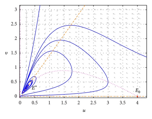
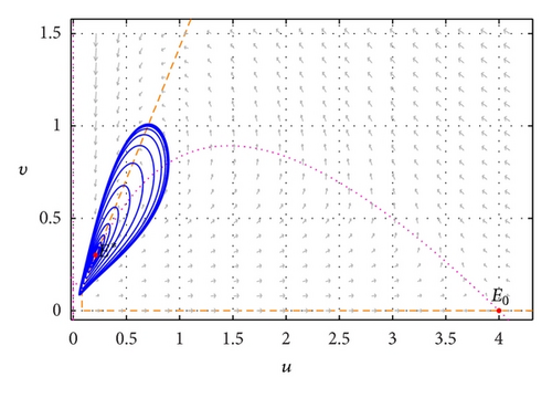
Figure 2 illustrates a Hopf-bifurcation situation of the model around E^* = (0.21053,0.30075) for s = s^* = 0.4912764003. In this case, limit cycle arising through Hopf bifurcation is a stable limit cycle which attracts all trajectories starting from a point in the interior of first quadrant.

2.3. The Stability of the Spatial Model (4)

In this subsection, we will focus on the effect of diffusion on the model system about the positive equilibrium.

Now, we study the nonlinear evolution of a perturbation

(20)

around E^* = (u^*, v^*). The corresponding linearized model (4) then takes the form

(21)

where a₁, a₂ are defined the same as (10).

We use [·, ·] to denote a column vector, and let

(22)

Let q = (q₁, q₂) ∈ Ω and

(23)

Then {e_q(x)} _q∈Ω forms a basis of the space of functions in ℝ² that satisfy zero-flux boundary conditions. We look for a normal mode corresponding to model (21) as following form:

(24)

where r_q is a vector depending on q. Plugging (24) into model (21) yields

(25)

where

. A nontrivial normal mode can be obtained by setting

(26)

This leads to the following dispersion formula for λ_q:

(27)

where

(28)

Mathematically speaking, a positive equilibrium E^* of model (4) is Turing unstable, which means that it is an asymptotically stable steady-state solution of the model (1) without diffusion but is unstable with respect to the solutions of the model (4) with diffusion.

Therefore, the Turing instability sets in when at least one of the following conditions is violated:

(29)

But it is evident that ρ₁ < 0 is not violated if s − a₁ < 0. Hence only the violation of condition ρ₂ > 0 gives rise to diffusion instability. As a consequence, a necessary condition is

(30)

Otherwise ρ₂ > 0 for all q > 0. For instability we must have ρ₂ < 0 for some q > 0, and we notice that ρ₂ achieves its minimum:

(31)

at the critical value

when

(32)

Summarizing the previous calculation, we conclude the following theorem.

Theorem 2. Assume that

(A1)
m(ar + cm + 2hr − acr) < r(a + h) ²(r + s + cs),
(A2)
r(a + h) ²(d₁s(1 + c) + d₂r) + 2 <d₂m(ar + cm + 2hr − acr).

Then the positive equilibrium E^* of model (4) is Turing unstable.

From Theorem 2, we can know that there is Turing instability in model (4) if conditions (A1) and (A2) hold. In this situation, the solutions to model (4) may be unstable and Turing patterns can emerge in the model.

3. Turing Pattern Formation

In this section, we perform extensive numerical simulations of the spatially extended model (4) in two-dimensional space, and the qualitative results are shown here. All our numerical simulations employ the zero-flux boundary conditions with a system size of 100 × 100. Other parameters are set as

(33)

The numerical integration of model (4) is performed by using a finite difference approximation for the spatial derivatives and an explicit Euler method for the time integration [35] with a time step size of 1/100. The initial condition is always a small amplitude random perturbation around the positive constant steady-state solution E^* = (u^*, v^*). After the initial period during which the perturbation spread, the model either goes to a time-dependent state or to an essentially steady-state solution (time independent).

We use the standard five-point approximation [36] for the 2D Laplacian with the zero-flux boundary conditions. More precisely, the concentrations

at the moment (n + 1)τ at the mesh position (x_i, y_j) are given by

(34)

with the Laplacian defined by

(35)

where f(u, v) = (ru(K − u)/(K + cu))−(muv/(u + av)), g(u, v) = sv(1 − (hv/u)), and the space step size e = 1/3.

In the numerical simulations, different types of dynamics are observed and it is found that the distributions of predator and prey are always of the same type. Consequently, we can restrict our analysis of pattern formation to one distribution. In this section, we show the distribution of prey u, for instance. We have taken some snapshots with red (blue) corresponding to the high (low) value of prey u.

Now, we show the Turing patterns for the different values of the control parameter s. Via numerical simulations, one can see that the model dynamics exhibits spatiotemporal complexity of pattern formation, including stripes, stripes-spots mixtures, and spots Turing patterns.

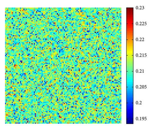
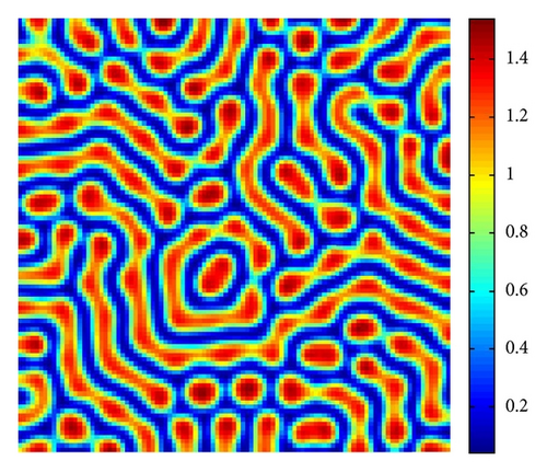
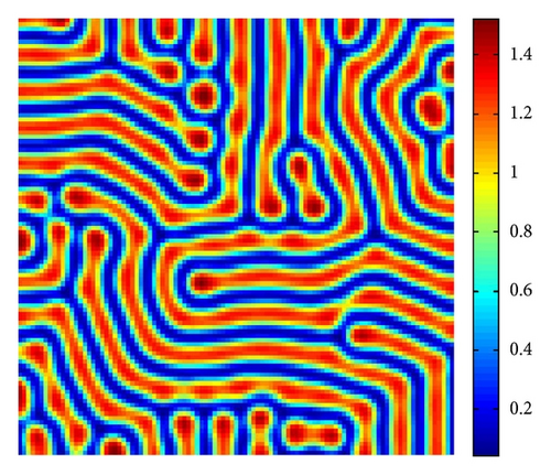
In Figure 3, with s = 1, starting with a homogeneous state E^* = (0.21,0.3) (cf. Figure 3(a)), the random perturbations lead to the formation to stripes spots (cf. Figure 3(c)), and the latter random perturbations make these spots decay, ending with the time-independent stripes pattern (cf. Figure 3(d)).

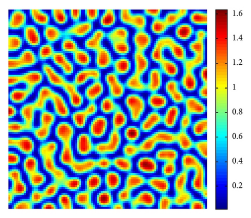
In Figure 4, with s = 1.375, we show the stripes-spots mixtures pattern for model (4).

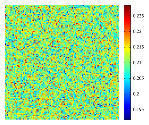
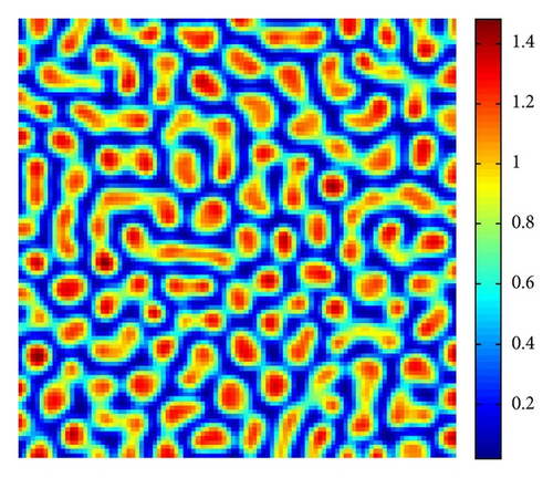
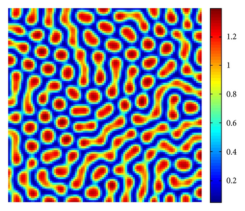
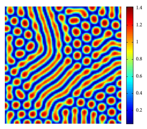
Figure 5 shows the time process of spots pattern formation of prey u for s = 2.5. In this case, the pattern takes a long time to settle down, starting with a homogeneous state E^* = (0.21,0.3) (cf. Figure 5(a)), and the random perturbations lead to the formation of stripes and spots (cf. Figure 5(b)), ending with spots only (cf. Figure 5(d))—the prey u is isolated zones with high population density, and the remainder region is of low density.

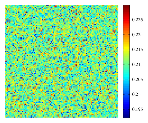
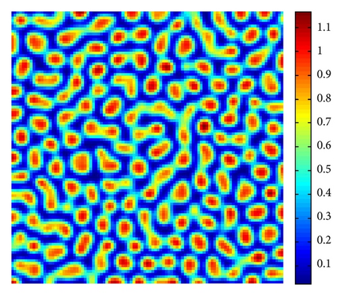
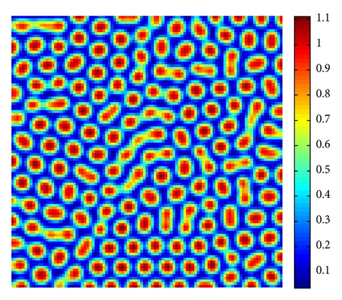
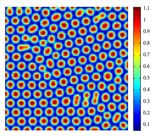
From Figure 3 to Figure 5, we can see that, on increasing the control parameter s from 1 to 2.5, the pattern sequence “stripe → stripes-spots mixtures → spots” can be observed.

4. Conclusions and Remarks

In summary, in this paper, we have investigated the spatiotemporal dynamics of a diffusive predator-prey model where the interaction between prey and predator follows Holling-Tanner formulation with ratio-dependent functional response and Smith growth. The value of this study is threefold. First, it presents the conditions for the stability of the equilibrium and the existence of Hopf bifurcation for the nonspatial model. Second, it rigorously proves Turing instability by linear stability analysis for the spatial model. Third, it illustrates the Turing pattern formation via numerical simulations, which shows that the spatial model dynamics exhibits complex pattern replication.

By a series of numerical simulations, we find that the spatial model (4) has rich Turing pattern replications, such as stripes, stripes-spots mixtures, and spots patterns. In the viewpoint of population ecology, in the case of stripe pattern (cf. Figure 3), the prey u is the isolated “stripes-like region” with high density, and the remainder stripes-like region is of low density. And in the case of spots pattern (cf. Figure 5), the prey u is the isolated “cycle region” with high density, and the remainder region is of low density, which is larger than the “spots” region.

References

1 Petrovskii S. V. and Malchow H., A minimal model of pattern formation in a prey-predator system, Mathematical and Computer Modelling. (1999) 29, no. 8, 49–63, https://doi.org/10.1016/S0895-7177(99)00070-9, MR1695498, ZBL0990.92040.
Google Scholar
2 Alonso D., Bartumeus F., and Catalan J., Mutual interference between predators can give rise to turing spatial patterns, Ecology. (2002) 83, no. 1, 28–34, 2-s2.0-0036141801.
Google Scholar
3 Turing A. M., The chemical basis of morphogenesis, Philosactions Transactions of the Royal Society of London. Series B. (1952) 237, no. 641, 37–72.
Google Scholar
4 Segel L. A. and Jackson J. L., Dissipative structure: an explanation and an ecological example, Journal of Theoretical Biology. (1972) 37, no. 3, 545–559, 2-s2.0-0015442349.
Google Scholar
5 Luckinbill L. S., The effects of space and enrichment on a predator-prey system, Ecology. (1974) 55, no. 5, 1142–1147.
Google Scholar
6 Levin S. A., The problem of pattern and scale in ecology: the Robert H. MacArthur award lecture, Ecology. (1992) 73, no. 6, 1943–1967.
10.2307/1941447
Google Scholar
7 Pascual M., Diffusion-induced chaos in a spatial predator-prey system, Proceedings of the Royal Society B. (1993) 251, no. 1330, 1–7, 2-s2.0-0027806283.
Google Scholar
8 Medvinsky A. B., Petrovskii S. V., Tikhonova I. A., Malchow H., and Li B.-L., Spatiotemporal complexity of plankton and fish dynamics, SIAM Review. (2002) 44, no. 3, 311–370, https://doi.org/10.1137/S0036144502404442, MR1951363, ZBL1001.92050.
Web of Science® Google Scholar
9 Murray J. D., Mathematical Biology. II: Spatial Models and Biomedical Applications, 2003, 18, 3rd edition, Springer, New York, NY, USA, Interdisciplinary Applied Mathematics, MR1952568.
Google Scholar
10 Peet A. B., Deutsch P. A., and Peacock-López E., Complex dynamics in a three-level trophic system with intraspecies interaction, Journal of Theoretical Biology. (2005) 232, no. 4, 491–503, https://doi.org/10.1016/j.jtbi.2004.08.028, MR2125828.
Google Scholar
11 Griffith D. A. and Peres-Neto P. R., Spatial modeling in ecology: the flexibility of eigenfunction spatial analyses, Ecology. (2006) 87, no. 10, 2603–2613, 2-s2.0-33845354872, https://doi.org/10.1890/0012-9658(2006)87%5b2603:SMIETF%5d2.0.CO;2.
Google Scholar
12 Pearce I. G., Chaplain M. A. J., Schofield P. G., Anderson A. R. A., and Hubbard S. F., Modelling the spatio-temporal dynamics of multi-species host-parasitoid interactions: heterogeneous patterns and ecological implications, Journal of Theoretical Biology. (2006) 241, no. 4, 876–886, https://doi.org/10.1016/j.jtbi.2006.01.026, MR2266757.
Google Scholar
13 Wang W., Liu Q.-X., and Jin Z., Spatiotemporal complexity of a ratio-dependent predator-prey system, Physical Review E. (2007) 75, no. 5, 9, 051913, https://doi.org/10.1103/PhysRevE.75.051913, MR2361820.
Web of Science® Google Scholar
14 Wang W., Zhang L., Wang H., and Li Z., Pattern formation of a predator-prey system with Ivlev-type functional response, Ecological Modelling. (2010) 221, no. 2, 131–140, 2-s2.0-70549086997, https://doi.org/10.1016/j.ecolmodel.2009.09.011.
Web of Science® Google Scholar
15 Wang W., Lin Y., Rao F., Zhang L., and Tan Y., Pattern selection in a ratio-dependent predator-prey model, Journal of Statistical Mechanics: Theory and Experiment. (2010) 2010, P11036.
Google Scholar
16 Wang W., Lin Y., Zhang L., Rao F., and Tan Y., Complex patterns in a predator-prey model with self and cross-diffusion, Communications in Nonlinear Science and Numerical Simulation. (2011) 16, no. 4, 2006–2015, https://doi.org/10.1016/j.cnsns.2010.08.035, MR2736066, ZBL1221.35423.
Google Scholar
17 Guan X., Wang W., and Cai Y., Spatiotemporal dynamics of a Leslie-Gower predator-prey model incorporating a prey refuge, Nonlinear Analysis: Real World Applications. (2011) 12, no. 4, 2385–2395, https://doi.org/10.1016/j.nonrwa.2011.02.011, MR2801027, ZBL1225.49038.
Google Scholar
18 Zhu Y., Cai Y., Yan S., and Wang W., Dynamical analysis of a delayed reaction-diffusion predator-prey system, Abstract and Applied Analysis. (2012) 2012, 23, 323186, MR2991022, ZBL1256.35183.
10.1155/2012/323186
Google Scholar
19 Cai Y., Wang W., and Wang J., Dynamics of a diffusive predator-prey model with additive Allee effect, International Journal of Biomathematics. (2012) 5, no. 2, 11, 1250023, https://doi.org/10.1142/S1793524511001659, MR2904442.
Web of Science® Google Scholar
20 Wang W., Guo Z., Upadhyay R. K., and Lin Y., Pattern formation in a cross-diffusive Holling-Tanner model, Discrete Dynamics in Nature and Society. (2012) 2012, 12, https://doi.org/10.1155/2012/828219, 828219.
10.1155/2012/828219
Web of Science® Google Scholar
21 Arditi R., Ginzburg L. R., and Akcakaya H. R., Variation in plankton densities among lakes: a case for ratio-dependent models, The American Naturalist. (1991) 138, no. 5, 287–1296.
Google Scholar
22 Arditi R. and Saiah H., Empirical evidence of the role of heterogeneity in ratio-dependent consumption, Ecology. (1992) 73, no. 5, 1544–1551, 2-s2.0-0027100815.
Google Scholar
23 Gutierrez A. P., Physiological basis of ratio-dependent predator-prey theory: the metabolic pool model as a paradigm, Ecology. (1992) 73, no. 5, 1552–1563, 2-s2.0-0027084787.
Google Scholar
24 Saha T. and Chakrabarti C., Dynamical analysis of a delayed ratio-dependent Holling-Tanner predator-prey model, Journal of Mathematical Analysis and Applications. (2009) 358, no. 2, 389–402, https://doi.org/10.1016/j.jmaa.2009.03.072, MR2532515, ZBL1177.34103.
Google Scholar
25 Arditi R. and Ginzburg L. R., Coupling in predator-prey dynamics: ratio-dependence, Journal of Theoretical Biology. (1989) 139, no. 3, 311–326, 2-s2.0-4944258042.
Google Scholar
26 Arditi R., Perrin N., and Saiah H., Functional responses and heterogeneities: an experimental test with cladocerans, Oikos. (1991) 60, no. 1, 69–75, 2-s2.0-0025946035.
Google Scholar
27 Liang Z. and Pan H., Qualitative analysis of a ratio-dependent Holling-Tanner model, Journal of Mathematical Analysis and Applications. (2007) 334, no. 2, 954–964, https://doi.org/10.1016/j.jmaa.2006.12.079, MR2338640, ZBL1124.34030.
Google Scholar
28 Banerjee M. and Banerjee S., Turing instabilities and spatio-temporal chaos in ratio-dependent Holling-Tanner model, Mathematical Biosciences. (2012) 236, no. 1, 64–76, https://doi.org/10.1016/j.mbs.2011.12.005, MR2902111.
Google Scholar
29 Smith F. E., Population dynamics in Daphnia Magna and a new model for population growth, Ecology. (1963) 44, 651–663.
Google Scholar
30 Pielou E. C., An Introduction to Mathematical Ecology, 1969, John Wiley & Sons, New York, NY, USA, MR0252051.
Google Scholar
31 Hallam T. G. and Deluna J. T., Effects of toxicants on populations: a qualitative approach III, Journal of Theoretical Biology. (1984) 109, no. 3, 411–429.
Google Scholar
32 Gopalsamy K., Kulenović M. R. S., and Ladas G., Environmental periodicity and time delays in a “food-limited” population model, Journal of Mathematical Analysis and Applications. (1990) 147, no. 2, 545–555, https://doi.org/10.1016/0022-247X(90)90369-Q, MR1050226, ZBL0701.92021.
Google Scholar
33 Feng W. and Lu X., On diffusive population models with toxicants and time delays, Journal of Mathematical Analysis and Applications. (1999) 233, no. 1, 373–386, https://doi.org/10.1006/jmaa.1999.6332, MR1684393, ZBL0927.35049.
Google Scholar
34 Fan M. and Wang K., Periodicity in a “food-limited” population model with toxicants and time delays, Acta Mathematicae Applicatae Sinica. (2002) 18, no. 2, 309–314, https://doi.org/10.1007/s102550200030, MR2008563, ZBL1025.34070.
Google Scholar
35 Garvie M. R., Finite-difference schemes for reaction-diffusion equations modeling predator-prey interactions in MATLAB, Bulletin of Mathematical Biology. (2007) 69, no. 3, 931–956, https://doi.org/10.1007/s11538-006-9062-3, MR2295839.
Google Scholar
36 Munteanu A. and Solé R. V., Pattern formation in noisy self-replicating spots, International Journal of Bifurcation and Chaos. (2006) 16, no. 12, 3679–3685, 2-s2.0-33847244910, https://doi.org/10.1142/S0218127406017063.
Google Scholar

Citing Literature

All articles

Pattern Formation in a Diffusive Ratio-Dependent Holling-Tanner Predator-Prey Model with Smith Growth

Abstract

1. Introduction

2. The Model and the Linear Stability Analysis

2.1. The Model

2.2. The Stability of the Nonspatial Model (1)

2.3. The Stability of the Spatial Model (4)

3. Turing Pattern Formation

4. Conclusions and Remarks

References

Citing Literature

Figures

References

Information

About Wiley Online Library

Help & Support

Opportunities

Connect with Wiley

Pattern Formation in a Diffusive Ratio-Dependent Holling-Tanner Predator-Prey Model with Smith Growth

Abstract

1. Introduction

2. The Model and the Linear Stability Analysis

2.1. The Model

2.2. The Stability of the Nonspatial Model (1)

2.3. The Stability of the Spatial Model (4)

3. Turing Pattern Formation

4. Conclusions and Remarks

References

Citing Literature

Figures

References

Related

Information