Volume 2013, Issue 1 270191

Research Article

Open Access

Complex Dynamics of a Diffusive Holling-Tanner Predator-Prey Model with the Allee Effect

Zongmin Yue,

Corresponding Author

Zongmin Yue

[email protected]

Faculty of Science, Shaanxi University of Science and Technology, Xi’an, Shaanxi 710021, China sust.edu.cn

Search for more papers by this author

Xiaoqin Wang,

Xiaoqin Wang

Faculty of Science, Shaanxi University of Science and Technology, Xi’an, Shaanxi 710021, China sust.edu.cn

Search for more papers by this author

Haifeng Liu,

Haifeng Liu

Faculty of Science, Shaanxi University of Science and Technology, Xi’an, Shaanxi 710021, China sust.edu.cn

Search for more papers by this author

Zongmin Yue,

Corresponding Author

Zongmin Yue

[email protected]

Faculty of Science, Shaanxi University of Science and Technology, Xi’an, Shaanxi 710021, China sust.edu.cn

Search for more papers by this author

Xiaoqin Wang,

Xiaoqin Wang

Faculty of Science, Shaanxi University of Science and Technology, Xi’an, Shaanxi 710021, China sust.edu.cn

Search for more papers by this author

Haifeng Liu,

Haifeng Liu

Faculty of Science, Shaanxi University of Science and Technology, Xi’an, Shaanxi 710021, China sust.edu.cn

Search for more papers by this author

First published: 11 February 2013

https://doi.org/10.1155/2013/270191

Citations: 3

Academic Editor: Lan Xu

Share a link

Email
Wechat
Bluesky

Abstract

We investigate the complex dynamics of a diffusive Holling-Tanner predation model with the Allee effect on prey analytically and numerically. We examine the existence of the positive equilibria and the related dynamical behaviors of the model and find that when the model is with weak Allee effect, the solutions are local and global stability for some conditions around the positive equilibrium. In contrast, when the model is with strong Allee effect, this may lead to the phenomenon of bistability; that is to say, there is a separatrix curve that separates the behavior of trajectories of the system, implying that the model is highly sensitive to the initial conditions. Furthermore, we give the conditions of Turing instability and determine the Turing space in the parameters space. Based on these results, we perform a series of numerical simulations and find that the model exhibits complex pattern replication: spots, spots-stripes mixtures, and stripes patterns. The results show that the impact of the Allee effect essentially increases the models spatiotemporal complexity.

1. Introduction

Recently, there has been a great interest in studying nonlinear difference/differential equations and systems [1–6]. One of the reasons for this is a necessity for some techniques which can be used in investigating equations arising in mathematical models describing real-life situations in population biology, economy, probability theory, genetics, psychology, sociology, and so forth. And the bases for analyzing the dynamics of complex ecological systems are the interactions between two species, particularly the dynamical relationship between predators and their preys [7]. From the Lotka-Volterra model [8, 9], several alternatives for modeling continuous time consumer-resource interactions have been proposed. In recent years, one of the important predator-prey models is Holling-Tanner model, which was described by May [10]. This model reads as follows:

()

where H and P represent prey and predator population densities at time t, respectively. r, K, c₁, k₁, s₁, and δ are positive constants. r₁ and s₁ are the intrinsic growth rate of prey and predator, respectively. K is the carrying capacity of the prey, and δ takes on the role of the prey-dependent carrying capacity for the predator. The rate at which the predator consumes the prey, c₁HP/(k₁ + H), is known as the Holling type-II functional response [11]. The parameter c₁ is the maximum number of the prey that can be eaten per predator per time, and k₁ is the saturation value that corresponds to the number of the preys necessary to achieve one half of the maximum rate c₁.

The dynamics of model (1) has been considered in many articles. For example, Hsu and Huang [12] obtained some results on the global stability of the positive equilibrium. More precise, under the conditions which local stability of the positive equilibrium implies its global stability. Gasull and coworkers [13] investigated the conditions of the asymptotic stability of the positive equilibrium which does not imply global stability. Sáez and González-Olivares [14] showed the asymptotic stability of a positive equilibrium and gave a qualitative description of the bifurcation curve.

On the other hand, in population dynamics, any mechanism that can lead to a positive relationship between a component of individual fitness and either the number or density of conspecifics constitutes what is usually called an Allee effect [15–24], starting with the pioneer work of Allee [25]. The outflux of prey to constant rate can be considered as Allee effect because a change on interaction dynamics is provoked, for instance, due to difficulty of encountering mates [17]. Nowadays, it is widely accepted that the Allee effect greatly increases the likelihood of local and global extinction [18] and can lead to a rich variety of dynamical effects.

From an ecological point of view, the Allee effect has been denominated in different ways [19–22] and modeled into strong and weak ones [15, 16, 19], depending on the degree of positive density dependence. Mathematically speaking, if H = H(t) indicates the population size, we assume that the growth function G(H) satisfies the following:

(i)
if G(0) = 0, G^′(0) > 0, G(H) is called weak Allee effect;
(ii)
if G(0) = 0, G^′(0) < 0, G(H) is called strong Allee effect.

The most common mathematical form describing this phenomenon for a single species is given by

()

where 0 < m < 1 or −1 < m ≤ 0, which is named the multiplicative Allee effect; here, a threshold value m is incorporated such that population growth is negative below m. When m < H < 1, the per capita growth rate is positive.

Furthermore, Boukal et al. [22] proposed that the prey exhibits a demographic Allee effect at low population densities due to reasons other than predation by the focal predator as follows:

()

where b is the Allee threshold, and c is an auxiliary parameter (c > 0 and b ≥ −c). The auxiliary parameter c affects the overall shape of the per capita growth curve of the prey. When c is fixed, the unit growth rate of the species is only in connection with the Allee threshold.

For model (1), we make a change of variables as follows:

()

For the sake of convenience, we still use variables H and P instead of

and

(H1) The basic model is a Holling-Tanner type as the form

()

where a = c₁/K, k₁ = K, and r = s₁/r.

(H2) Following Boukal et al. [22], in Allee effect equation (3), we choose the auxiliary parameter c = 1, and b + 1 ≡ m is the Allee threshold. That is, prey H has the population growth function

()

Obviously, we have the following:

(i)
if 0 < m ≤ 1, G(0) = 0, G^′(0) > 0, the Allee effect (6) is the weak one;
(ii)
if m > 1, G(0) = 0, G^′(0) < 0, the Allee effect (6) is the strong one;
(iii)
if m = 0, the Allee effect will disappear.

And we can get the following model with the Allee effect on prey:

()

(H3) Assume that the individuals in populations H and P move randomly described as Brownian random motion [26]. We can get a simple spatial model corresponding to model (7) as follows:

()

Here, the nonnegative constants d₁ and d₂ are the diffusion coefficients of H(t) and P(t), respectively. ∇² = ∂²/∂x² + ∂²/∂y² is the Laplacian operator in two-dimensional space, which describes the random moving. The initial distribution of species N₀ and P₀ are continuous functions. And the boundary condition is assumed to be zero-flux one as follows:

()

L indicates the size of the model in the directions of x and y, respectively, and n is the outward unit normal vector of the boundary ∂Ω. The main reason for choosing such boundary conditions is that we are interested in the self-organization of pattern, and the zero-flux boundary conditions imply that no external input is imposed form exterior [27].

There are some excellent works on a Holling-Tanner model considering the diffusion [28–33] and the references therein. In [28], Guan and co-workers studied the spatiotemporal dynamics of a modified version of the Leslie-Gower predator-prey model incorporating a prey refuge and showed that the model dynamics exhibits complex Turing pattern replication: stripes, cold/hot spots-stripes coexistence, and cold/hot spots patterns. Without the Allee effect, Peng and Wang [29, 30] analyzed the global stability of the unique positive constant steady state and established some results for the existence and nonexistence of positive nonconstant steady states. Wang et al. [31] considered the Turing and Hopf bifurcations of the equilibrium solutions. Liu and Xue [32] investigated the pattern formation and found that spots, black-eye, and labyrinthine patterns can be observed in the model. Chen and Shi [33] proved global stability of the unique constant equilibrium.

However, the research about the influence of Allee effect on pattern formation of diffusive Holling-Tanner model seems rare. The main purpose of this paper is to study dynamical behaviors of a Holling-Tanner predator-prey model with the Allee effect. We will determine how the Allee effect affects the dynamics of the model and focus on the stability of the positive steady state and bifurcation mechanism and patterns formation analysis of the model.

The rest of the paper is organized as follows. In Sections 2 and 3, we present our main results about the stability and bifurcation analysis of the nonspatial model (7) and the spatial model (8), respectively. Especially, in regards to the spatial model (8) in Section 3, we will give the conditions of the Turing instability and determine the Turing space, and by performing a series of numerical simulations, we illustrate the emergence of different patterns. Finally, in Section 4, some conclusions and remarks are given.

2. Dynamics Analysis of the Nonspatial Model (7)

2.1. Boundedness

Now, we prove that all solutions are eventually bounded.

Theorem 1. All the solutions of model (7) which are initiated in are uniformly bounded.

Proof. Let H(t) and P(t) be any solution of model (7) with initial conditions (H(0), P(0)) = (H₀, P₀) such that H₀ > 0, P₀ > 0. From the first equation of model (7), we have

()

a standard comparison theorem shows that

()

Then, from the second equation of model (7), we get dP/dt ≤ rP(1 − (P/δ)), which implies that

()

Define the function W(t) = H(t) + P(t), differentiating both sides with respect to t; we get

()

Then,

()

Using the theory of differential inequality, for all t ≥ T ≥ 0, we have

()

Hence, limsup _t→∞ (H(t) + P(t)) ≤ M. This completes the proof.

Remark 2. In fact, if m ≥ 2, dH/dt < 0 always holds, which means that the prey and predator will extinct. Hence, we will later only focus on the case of 0 ≤ m < 2.

Next, we will investigate the existence of equilibria and their local and global stability with respect to model (7).

2.2. Equilibria Analysis in the Case of the Strong Allee Effect (i.e., 1 < m < 2)

In this subsection, we consider the existence and stability of the equilibrium of model (7) with strong Allee effect; that is, 1 < m < 2.

We note that model (7) is not defined at the P-axis, particularly at the point (0,0), but both isoclines pass through this point, and in this case, it is a point of particular interest [34]. The character of (0,0) can be obtained after rescaling the time in model (7) by t = τH(1 + H) as follows:

()

Lemma 3. The point (0,0) of model (16) has a hyperbolic and a parabolic sector [20, 35] determined for the line P = (δ(m − 1 + r)/r)H. That is, there exists a separatrix curve in the phase plane that divides the behavior of trajectories; the point (0,0) is then an attractor point for certain trajectories and a saddle point for others.

Proof. As the Jacobian matrix of the point (0,0) for model (16) is the zero matrix, we follow the methodology used in [20, 35] given by the function φ(u, v) = (uv, v) = (H, P). Then, we have that

()

and rescaling the time by T = vτ, it becomes

()

Clearly, if v = 0, then dv/dT = 0. Moreover, du/dT = u((1 − m)u − r(u − (1/δ))).

The singularities of model (18) are (0,0) and (r/(δ(m − 1 + r)), 0); that is, a separatrix straight exists in the phase plane uv, given by u = r/(δ(m − 1 + r)). The Jacobian matrixes of (0,0) and (r/(δ(m − 1 + r)), 0) for model (18) are

()

Then, (0,0) is a hyperbolic saddle point, and (r/(δ(m − 1 + r)), 0) is an attractor point. Using the blowing down, the point (0,0) is a saddle node in model (16), and the line P = ((δ(m − 1 + r))/r)H divides the behavior of trajectories on the phase plane. The proof is completed.

Moreover, it is easy to verify that model (7) always has two boundary equilibria E₀ = (m − 1,0) and E₁ = (1,0). And the behavior of model (7) around E₀ and E₁ is found as follows.

The Jacobian matrix of model (7) at the equilibrium E₀ = (m − 1,0) takes the form

()

Hence, the equilibrium E₀ = (m − 1,0) is an unstable node point (nodal source).

The Jacobian matrix of model (7) at the equilibrium E₀ = (1,0) takes the form

()

Hence, the equilibrium E₁ = (1,0) is a saddle point.

And model (7) has a positive equilibrium E = (H, δH), where H satisfies

()

For simplicity, we consider A = m − aδ and

; then, the two roots of (22) are given by

()

Lemma 4.

(i)
Suppose that m − aδ > 0 and 1 < m < 2.
- (a)
  If B² > 0 holds, model (7) has two positive equilibria E₊ = (H₊, δH₊) and E₋ = (H₋, δH₋).
- (b)
  If B² = 0 holds, model (7) has a unique positive equilibrium E_e = (H_e, δH_e). Note that in this case .
- (c)
  If B² < 0, model (7) has no positive equilibrium.
(ii)
If m − aδ ≤ 0, model (7) has no positive equilibrium.

Let E = (N, P) be an arbitrary positive equilibrium. The Jacobian matrix of model (7) at the positive equilibrium E = (H, δH) takes the form

()

Then, we can get

()

We can see that the sign of det (J_E) is determined by

()

Thus, we can obtain

()

Hence, we obtain , , and . And the positive equilibrium E₋ = (H₋, δH₋) is a saddle point. The nature of the equilibrium point E₊ is dependent on the sign of the trace of the Jacobian matrix evaluated in this point. Whether E₊ is a node or a focus depends on the sign of .

In the following results, we study the stability of the positive equilibrium E₊ and the unique positive equilibria E_e.

Theorem 5. Define

()

(a)
If r > r₊, the positive equilibrium E₊ = (H₊, δH₊) is a locally asymptotically stable point;
- (a1)
  if , then E₊ is a stable focus,
- (a2)
  if , then E₊ is a stable node point.
(b)
If r < r₊, the positive equilibrium E₊ = (H₊, δH₊) is an unstable point;
- (b1)
  if , then E₊ is an unstable focus surrounded by a stable limit cycle,
- (b2)
  if , then E₊ is an unstable node and the limit cycle disappears.
(c)
A Hopf bifurcation occurs at r = r₊ around the positive equilibrium E₊ = (H₊, δH₊). That is to say, model (7) has at least one positive periodic orbit.

Proof. Here, we only give the proof of the existence of Hopf bifurcation. It is easy to see that

(i)
holds,
(ii)
the characteristic equation is , whose roots are purely imaginary,
(iii)
.

From the Poincaré-Andronov-Hopf Bifurcation Theorem [36], we know that model (7) undergoes a Hopf bifurcation at E₊ as r passes through the value r₊. The proof is completed.

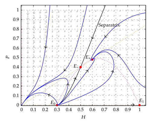
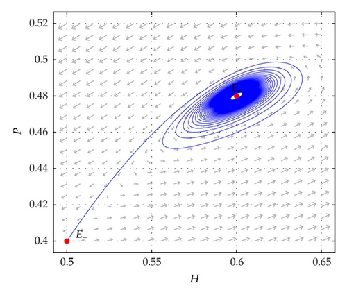
Figure 1 illustrates the local stability of the positive equilibrium E₊ and the separatrix curve generated by the stable manifold of the positive equilibrium E₋. The orbits initiating the right of the separatrix curve tend to E₊, while the orbits initiating the left of the separatrix curve tend to (0,0) that represents the extinction of the population. Figure 2 illustrates a Hopf bifurcation situation of the model around E₊. The parameter values are given in the figures.

Details are in the caption following the image — **Figure 1**
Open in figure viewer PowerPoint

The phase portrait of model (7) with the strong Allee effect. The parameters are taken as a = 0.25, δ = 0.8, m = 1.3 and r = 0.15. In this case, E₀ = (0.3,0) is an unstable node point, E₁ = (1,0) and E₋ = (0.5, 0.4) are saddle points; the positive equilibrium E₊ = (0.6, 0.48) is local asymptotically stable. There exists a separatrix curve determined by the stable manifold of the equilibrium point E₋. The dotted curves are the nullclines.

Theorem 6. The unique equilibrium point is

(i)
a nonhyperbolic attractor node, if and only if ;
(ii)
a nonhyperbolic repellor node, if and only if ;
(iii)
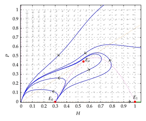
a cusp point, if and only if , and in this case, there exists a unique trajectory which attains the point E_e. And in this case, the point (0,0) is a global attractor.

Proof. We have

()

Hence (i) and (ii) hold.

Moreover, , if and only if . In this case, we obtain the Jacobian matrix of (16) as follows:

()

and the associate Jordan matrix is

()

Then, the singularity

is a cusp point, since it is a point of codimension 2, and we have a Bogdanov-Takens bifurcation [37].

The cusp point is shown in Figure 3.

2.3. Equilibria Analysis in the Case of the Weak Allee Effect (i.e., 0 < m ≤ 1)

In this subsection, we consider the stability of the equilibrium of model (7) with weak Allee effect (0 < m ≤ 1).

It is easy to verify that model (7) always has one boundary equilibrium E₀ = (1,0) which is a saddle point and a positive equilibrium E^* = (H^*, δH^*), where

()

From (24), we have

()

Hence, we have the following results on the stability of the positive equilibrium E^* = (H^*, δH^*).

Theorem 7. Define

()

(a)
If r > r^*, the positive equilibrium E^* = (H^*, δH^*) is a locally asymptotically stable point, and
- (a1)
  if , then E^* is a stable focus;
- (a2)
  if , then E^* is a stable node point.
(b)
If r < r^*, the positive equilibrium E^* = (H^*, δH^*) is an unstable point, and
- (b1)
  if , then E^* is an unstable focus surrounded by a stable limit cycle;
- (b2)
  if , then E^* is an unstable node and the limit cycle disappears.
(c)
A Hopf bifurcation occurs at r = r^* around the positive equilibrium E^* = (H^*, δH^*). That is to say, model (7) has at least one positive periodic orbit.

In the following theorem, we study the global behavior of the positive equilibrium E^*.

Theorem 8. If 0 < m < 1/(1 + aδ), the positive equilibrium E^* = (H^*, δH^*) is globally asymptotically stable.

Proof. Construct the following Lyapunov function:

()

where

()

Then,

()

Substituting the value of dH/dt and dP/dt from the model of (7), we obtained

()

Note that aδH^* = H^*(1 − H^*)(1 + H^* − m); we obtain

()

Hence, if 0 < m < 1/(1 + aδ), H^* − m > 0 which is equivalent to dV/dt < 0.

Hence, the positive equilibrium E^* = (H^*, δH^*) is globally asymptotically stable. This completes the proof.

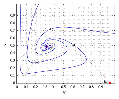
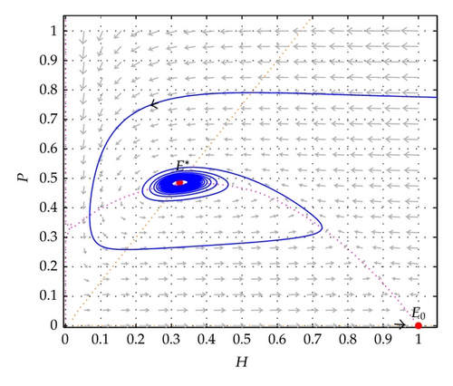
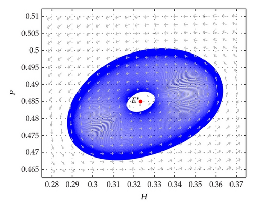
Figure 4 demonstrates the global stability situation of model (7) around E^*. Figure 5 illustrates a Hopf bifurcation situation of the model around E^*. Figure 6 shows a stable limit cycle around E^* which is an unstable focus. The parameter values are given in the figures.

3. Dynamics of the Spatial Model (8)

In this section, we will investigate the dynamics of the spatial model (8). As an example, we only focus on the positive equilibrium point E^* = (H^*, δH^*) in the case of weak Allee effect (0 < m < 1).

3.1. Turing Instability

Mathematically speaking, an equilibrium is Turing instability (diffusion-driven instability) means that it is an asymptotically stable equilibrium E^* of model (7) but is unstable with respect to the solutions of reaction-diffusion model (8).

In the presence of diffusion, we will introduce small perturbations U₁ = H − H^*, U₂ = P − δH^*, where |U₁ | , |U₂ | ≪ 1. To study the effect of diffusion on the model, we have considered the linearized form of model as follows:

()

where r^* is defined as (34).

Following Malchow et al. [38], we can know that any solution of model (40) can be expanded into a Fourier series so that

()

where r = (x, y), and 0 < x < L and 0 < y < L. k = (k_n, k_m), and k_n = nπ/L and k_m = mπ/L are the corresponding wavenumbers.

Having substituted u_nm and v_nm into (40), we obtain

()

where

A general solution of (42) has the form C₁exp (λ₁t) + C₂exp (λ₂t), where the constants C₁ and C₂ are determined by the initial conditions (3), and the exponents λ₁ and λ₂ are the eigenvalues of the following matrix:

()

Correspondingly, λ₁ and λ₂ are the solutions of the following equation:

()

where

()

Summarizing the previous discussions, we can get the following theorem immediately.

Theorem 9. (i) The positive equilibrium E^* of model (8) is locally asymptotically stable if r > max {r^*, r^*d₂/d₁} holds.

(ii) If the positive equilibrium E^* of model (7) is globally asymptotically stable, then the corresponding steady state E^* of model (8) is also globally asymptotically stable.

Proof. (i) Using Routh-Hurwitz criteria, we can know that the positive equilibrium E^* is locally asymptotically stable, if and only if and . So, we obtain r > max {r^*, r^*d₂/d₁}.

(ii) We select the Lyapunov function for model (8) as follows:

()

where V(H, P) is the same as defined in (35). So,

()

Using Green’s first identity in the plane,

()

Considering the zero-flux boundary conditions, one can show that

()

From the previous analysis, we note that dV₂/dt < 0 is valid if dV/dt < 0 is true. This implies that the equilibrium E^* of both model (7) and model (8) is globally asymptotically stable if 0 < m < 1/(1 + aδ) holds. This ends the proof.

On the other hand, Turing instability sets in when at least one of the conditions is either

. It is evident that the condition

is not violated when the requirement r^* − r < 0 is met [39]. Hence, only violation of condition

gives rise to diffusion instability. Then, the condition for diffusive instability is given by

()

G(·) is quadratic in k², and the graph of G(k²) = 0 is a parabola. The minimum of G(k²) occurs at

, where

()

The critical wave number k_c of the first perturbations to grow is found by evaluating k_m from (51).

Thus, a sufficient condition for Turing instability is that

is negative. Therefore,

()

Combination of (51) and (52) leads to the following final criterion for diffusive instability:

()

Summarizing the previous discussions, we can obtain the following theorem.

Theorem 10. If rd₁/d₂ < r^* < r and hold, the criterion for Turing instability for model (8) emerges, and the critical wave number .

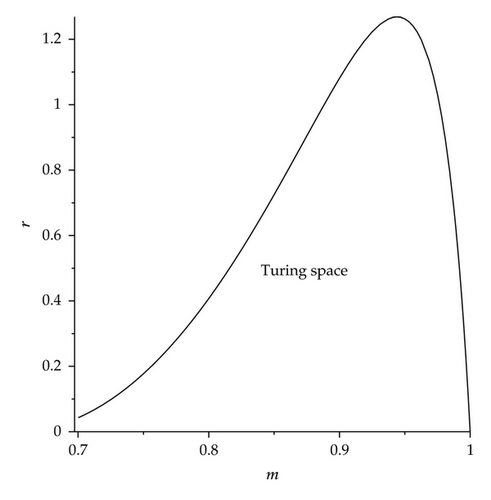
The Turing instability (or bifurcation) breaks spatial symmetry, leading to the formation of patterns that are stationary in time and oscillatory in space [40, 41]. We adopt the intrinsic growth rates of predator r as the bifurcation parameter, and the linear stability analysis yields the bifurcation diagram shown in Figure 7. The Turing bifurcation curve separates the parametric space into two domains. Above the curve, the solutions of model (8) are stable for all pairs of (m, r); that is, there is no Turing instability. While below the curve, the solutions of model (8) are unstable for (m, r) and diffusive instability emerges; that is, Turing patterns emerge. This domain is called the Turing space.

3.2. Pattern Formation

In this subsection, we performed extensive numerical simulations of the spatially extended model (8) in two-dimension spaces, and the qualitative results are shown here. All our numerical simulations employ the zero-flux boundary conditions with a model size of L × L, with L = 100 discretized through x → (x₀, x₁, x₂, …, x_n) and y → (y₀, y₁, y₂, …, y_n), with n = 200. Other parameters are fixed as a = 0.8, δ = 1.75, r = 0.15, d₁ = 0.01, and d₂ = 1.

The numerical integration of model (8) is performed by using a finite difference approximation for the spatial derivatives and an explicit Euler method for the time integration [42] with a time stepsize of τ = 1/100. The initial condition is always a small amplitude random perturbation around the positive constant steady state solution E^*. After the initial period during which the perturbation spread, either the model goes into a time-dependent state or to an essentially steady state solution (time independent).

More precisely, the concentrations

at the moment (n + 1)τ at the mesh position (i, j) are given by

()

with the Laplacian defined by

()

where f(H, P) = H(1 − H)(1 − m/(H + 1)) − aHP/(1 + H), g(H, P) = rP(1 − P/δH), and the space stepsize h = 1/3.

In the numerical simulations, different types of dynamics are observed, and it is found that the distributions of predator and prey are always of the same type. Consequently, we can restrict our analysis of pattern formation to one distribution. In this section, we show the distribution of prey H, for instance.

Figure 8 shows the evolution of the spatial pattern of prey H at t = 0, 500, 1000, 2000, with small random perturbation of the stationary solution E^* of the spatially homogeneous systems when m is located in “Turing space.” In this case, one can see that for model (8), the random initial distribution leads to the formation of a strongly irregular transient pattern in the domain. After the irregular pattern is formed (c.f., Figures 8(b) and 8(c)), it grows slightly and jumps alternately for a certain time, and finally spots patterns, which are isolated zones with low prey densities, prevail over the whole domain, and the dynamics of the model does not undergo any further changes (c.f., Figure 8(d)).

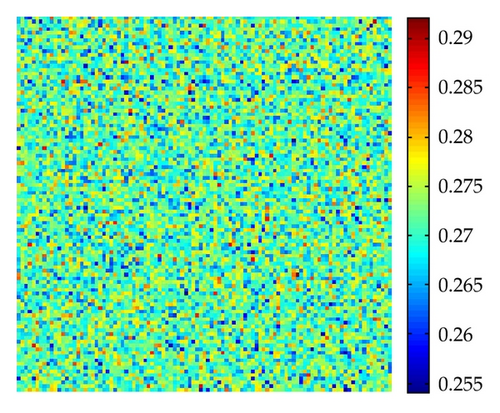
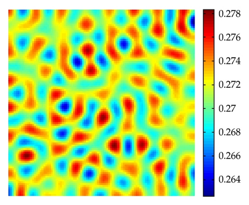
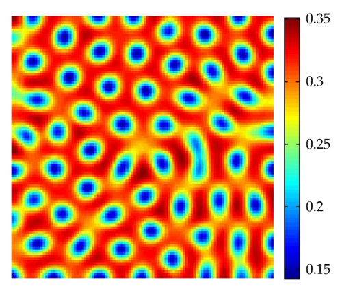
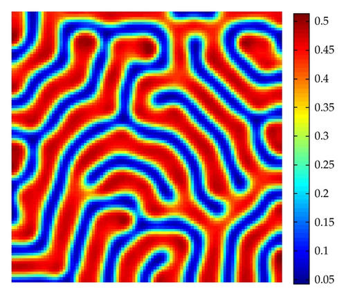
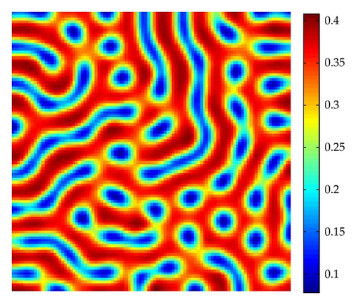
Figure 9 shows stripe patterns are interlaced stripes of high and low population densities of prey H for the parameter m = 0.78 at t = 1000. In Figure 10, with the parameter m = 0.85, the spot-stripe mixtures pattern is time independent with low prey densities.

4. Concluding Remarks

In this paper, we are concerned with the complex dynamics in a diffusive Holling-Tanner predator-prey model with the Allee effect on prey. The value of this study lies in two folds. First, the local asymptotic stability conditions for coexisting equilibrium and conditions for Hopf bifurcation are described briefly for the model with the weak and strong Allee effects. Second, it gives the analysis of Turing instability which determines the Turing space in the spatial domain and meanwhile illustrates the Turing pattern formation close to the onset Turing bifurcation via numerical simulations, which shows that the model dynamics exhibits complex pattern replication.

We note that in the analyzed models, a big difference between the dynamics of model with strong or weak Allee effect exists. In the case of strong Allee effect, two positive equilibria can coexist for a subset of parameters with a varied dynamics but different to other Holling-Tanner models analyzed earlier [12–14]. We have shown that one of these equilibria is always a saddle point and proved the existence of a separatrix curve. And there is no global asymptotically stable positive equilibrium. In this case, the point (0,0) is an attractor in addition to locally stable positive equilibrium E₊ for determined parameter values, which leads to the existence of a bistability phenomenon. The dynamics of the model is determined by the initial conditions; the predator and prey may be extinction or coexistence. This means that the strong Allee effect could easily lead to the risk of population extinction. Nevertheless, in the case of weak Allee effect, model (7) can only have one unique positive equilibrium, which is globally asymptotically stable under some conditions. Therefore, the predators and preys can coexist in stable conditions.

Furthermore, we have investigated the conditions for the predator-prey model which experiences spatial patterns through diffusion-driven instability. We have derived the conditions of Turing instability in terms of our model parameters analytically. In addition, to get a deeper insight into the model’s dynamics behaviour, we select the different values of parameter m. An increase of m, from the numerical results, one can see that our model has rich and complex spatiotemporal behavior. We find three typical Turing patterns, that is, spots pattern, stripes pattern, and spots-stripes mixtures pattern. To the best of our knowledge, the Turing pattern we illustrate here is the first reported case to our model. And our complete analysis of the spatial model will give new suggestion to the models with the Allee effect.

Acknowledgments

The authors would like to thank the anonymous referee for very helpful suggestions and comments which led to improvements of their original paper. And this work is supported by the Cooperative Project of Yulin City (2011).

References

1 Murray J. D., Mathematical Biology. II: Spatial Models and Biomedical Applications, 2003, 18, 3rd edition, Springer, New York, NY, USA, Interdisciplinary Applied Mathematics, MR1952568, ZBL1137.62393.
10.1007/b98869
Google Scholar
2 Stević S., A short proof of the Cushing-Henson conjecture, Discrete Dynamics in Nature and Society. (2006) 5, 37264, https://doi.org/10.1155/DDNS/2006/37264, MR2272408, ZBL1149.39300.
10.1155/DDNS/2006/37264
Web of Science® Google Scholar
3 Stević S., Asymptotic behavior of a class of nonlinear difference equations, Discrete Dynamics in Nature and Society. (2006) 10, 47156, https://doi.org/10.1155/DDNS/2006/47156, MR2261037, ZBL1121.39006.
10.1155/DDNS/2006/47156
Web of Science® Google Scholar
4 De La Sen M. and Alonso-Quesada S., Model-matching-based control of the Beverton-Holt equation in ecology, Discrete Dynamics in Nature and Society. (2008) 21, 793512, https://doi.org/10.1155/2008/793512, MR2385395, ZBL1149.92029.
10.1155/2008/793512
Web of Science® Google Scholar
5 De la Sen M. and Alonso-Quesada S., A control theory point of view on Beverton-Holt equation in population dynamics and some of its generalizations, Applied Mathematics and Computation. (2008) 199, no. 2, 464–481, https://doi.org/10.1016/j.amc.2007.10.021, MR2420576, ZBL1137.92034.
10.1016/j.amc.2007.10.021
Web of Science® Google Scholar
6 He J., Asymptotic methods for solitary solutions and compactons, Abstract and Applied Analysis. (2012) 2012, 130, 916793, https://doi.org/10.1155/2012/916793.
10.1155/2012/916793
Google Scholar
7 Li Y. and Xiao D., Bifurcations of a predator-prey system of Holling and Leslie types, Chaos, Solitons & Fractals. (2007) 34, no. 2, 606–620, https://doi.org/10.1016/j.chaos.2006.03.068, MR2327437, ZBL1156.34029.
10.1016/j.chaos.2006.03.068
Web of Science® Google Scholar
8 Lotka A. J., Elements of Physical Biology, 1925, Williams and Wilkins, Baltimore, Md, USA.
Web of Science® Google Scholar
9 Volterra V., Fluctuations in the abundance of a species considered mathematically, Nature. (1926) 118, no. 2972, 558–560, 2-s2.0-0006170098.
10.1038/118558a0
Web of Science® Google Scholar
10 May R. M., Stability and Complexity in Model Ecosystems, 1974, Princeton University Press, Princeton, NJ, USA.
Google Scholar
11 Holling C. S., The components of predation as revealed by a study of small-mammal predation of the European Pine Sawfly, The Canadian Entomologist. (1959) 91, no. 5, 293–320.
10.4039/Ent91293-5
Web of Science® Google Scholar
12 Hsu S. B. and Huang T. W., Global stability for a class of predator-prey systems, SIAM Journal on Applied Mathematics. (1995) 55, no. 3, 763–783, https://doi.org/10.1137/S0036139993253201, MR1331585, ZBL0832.34035.
10.1137/S0036139993253201
Web of Science® Google Scholar
13 Gasull A., Kooij R. E., and Torregrosa J., Limit cycles in the Holling-Tanner model, Publicacions Matematiques. (1997) 41, no. 1, 149–167.
10.5565/PUBLMAT_41197_09
Google Scholar
14 Sáez E. and González-Olivares E., Dynamics of a predator-prey model, SIAM Journal on Applied Mathematics. (1999) 59, no. 5, 1867–1878, https://doi.org/10.1137/S0036139997318457, MR1710547, ZBL0934.92027.
10.1137/S0036139997318457
Web of Science® Google Scholar
15 Wang G., Liang X. G., and Wang F. Z., The competitive dynamics of populations subject to an Allee effect, Ecological Modelling. (1999) 124, no. 2-3, 183–192, 2-s2.0-0033552648, https://doi.org/10.1016/S0304-3800(99)00160-X.
10.1016/S0304-3800(99)00160-X
Web of Science® Google Scholar
16 Kent A., Doncaster C. P., and Sluckin T., Consequences for predators of rescue and Allee effects on prey, Ecological Modelling. (2003) 162, no. 3, 233–245, 2-s2.0-0037446297, https://doi.org/10.1016/S0304-3800(02)00343-5.
10.1016/S0304-3800(02)00343-5
Web of Science® Google Scholar
17 Gonzalez-Olivares E., Mena-Lorca J., Meneses-Alcay H., Gonzalez-Yanez B., and Flores J. D., Allee effect, emigration and immigration in a class of predator-prey models, Biophysical Reviews and Letters. (2008) 3, 195–251.
10.1142/S1793048008000691
Google Scholar
18 Zhou S. R., Liu Y. F., and Wang G., The stability of predator-prey systems subject to the Allee effects, Theoretical Population Biology. (2005) 67, no. 1, 23–31, 2-s2.0-11844279070, https://doi.org/10.1016/j.tpb.2004.06.007.
10.1016/j.tpb.2004.06.007
PubMed Web of Science® Google Scholar
19 Wang J., Shi J., and Wei J., Predator-prey system with strong Allee effect in prey, Journal of Mathematical Biology. (2011) 62, no. 3, 291–331, https://doi.org/10.1007/s00285-010-0332-1, MR2771175, ZBL1232.92076.
10.1007/s00285-010-0332-1
PubMed Web of Science® Google Scholar
20 González-Olivares E., Mena-Lorca J., Rojas-Palma A., and Flores J. D., Dynamical complexities in the Leslie-Gower predator-prey model as consequences of the Allee effect on prey, Applied Mathematical Modelling. (2011) 35, no. 1, 366–381, https://doi.org/10.1016/j.apm.2010.07.001, MR2677950, ZBL1202.34079.
10.1016/j.apm.2010.07.001
Web of Science® Google Scholar
21 Aguirre P., González-Olivares E., and Sáez E., Three limit cycles in a Leslie-Gower predator-prey model with additive Allee effect, SIAM Journal on Applied Mathematics. (2009) 69, no. 5, 1244–1262, https://doi.org/10.1137/070705210, MR2487059, ZBL1184.92046.
10.1137/070705210
Web of Science® Google Scholar
22 Boukal D. S., Sabelis M. W., and Berec L., How predator functional responses and Allee effects in prey affect the paradox of enrichment and population collapses, Theoretical Population Biology. (2007) 72, no. 1, 136–147, 2-s2.0-34249935507, https://doi.org/10.1016/j.tpb.2006.12.003.
10.1016/j.tpb.2006.12.003
PubMed Web of Science® Google Scholar
23 Cai Y., Wang W., and Wang J., Dynamics of a diffusive predator-prey model with additive Allee effect, International Journal of Biomathematics. (2012) 5, no. 2, 1250023, https://doi.org/10.1142/S1793524511001659, MR2904442.
10.1142/S1793524511001659
Web of Science® Google Scholar
24 Morozov A., Petrovskii S., and Li B. L., Bifurcations and chaos in a predator-prey system with the Allee effect, Proceedings of the Royal Society B. (2004) 271, no. 1546, 1407–1414, 2-s2.0-3042846003, https://doi.org/10.1098/rspb.2004.2733.
10.1098/rspb.2004.2733
PubMed Web of Science® Google Scholar
25 Allee W. C., Animal Aggregations: A Study in General Sociology, 1931, University of Chicago Press, Chicago, Ill, USA.
10.5962/bhl.title.7313
Google Scholar
26 Cantrell R. S. and Cosner C., Spatial Ecology via Reaction-Diffusion Equations, 2003, John Wiley & Sons, Chichester, UK, Wiley Series in Mathematical and Computational Biology, https://doi.org/10.1002/0470871296, MR2191264.
10.1002/0470871296
Google Scholar
27 Murray J. D., Discussion: turing’s theory of morphogenesis-its influence on modelling biological pattern and form, Bulletin of Mathematical Biology. (1990) 52, no. 1-2, 119–132.
10.1016/S0092-8240(05)80007-2
Web of Science® Google Scholar
28 Guan X., Wang W., and Cai Y., Spatiotemporal dynamics of a Leslie-Gower predator-prey model incorporating a prey refuge, Nonlinear Analysis: Real World Applications. (2011) 12, no. 4, 2385–2395, https://doi.org/10.1016/j.nonrwa.2011.02.011, MR2801027, ZBL1225.49038.
10.1016/j.nonrwa.2011.02.011
Web of Science® Google Scholar
29 Peng R. and Wang M., Positive steady states of the Holling-Tanner prey-predator model with diffusion, Proceedings of the Royal Society of Edinburgh A. (2005) 135, no. 1, 149–164, https://doi.org/10.1017/S0308210500003814, MR2119846, ZBL1144.35409.
10.1017/S0308210500003814
Web of Science® Google Scholar
30 Peng R. and Wang M., Global stability of the equilibrium of a diffusive Holling-Tanner prey-predator model, Applied Mathematics Letters. (2007) 20, no. 6, 664–670, https://doi.org/10.1016/j.aml.2006.08.020, MR2314410, ZBL1125.35009.
10.1016/j.aml.2006.08.020
Web of Science® Google Scholar
31 Wang W., Lin Y., Zhang L., Rao F., and Tan Y., Complex patterns in a predator-prey model with self and cross-diffusion, Communications in Nonlinear Science and Numerical Simulation. (2011) 16, no. 4, 2006–2015, https://doi.org/10.1016/j.cnsns.2010.08.035, MR2736066, ZBL1221.35423.
10.1016/j.cnsns.2010.08.035
Web of Science® Google Scholar
32 Liu P. and Xue Y., Spatiotemporal dynamics of a predator-prey model, Nonlinear Dynamics. (2012) 69, no. 1-2, 71–77.
10.1007/s11071-011-0246-5
Web of Science® Google Scholar
33 Chen S. and Shi J., Global stability in a diffusive Holling-Tanner predator-prey model, Applied Mathematics Letters. (2012) 25, no. 3, 614–618, https://doi.org/10.1016/j.aml.2011.09.070, MR2856044.
10.1016/j.aml.2011.09.070
Web of Science® Google Scholar
34 Mena-Lorca J., Gonzalez-Olivares E., and Gonzalez-Yanez B., The Leslie-Gower predator-prey model with Allee effect on prey: a simple model with a rich and interesting dynamiscs, Proceedings of the International Symposium on Mathematical and Computational Biology, 2006, 105–132.
Google Scholar
35 Sáez E. and González-Olivares E., Dynamics of a predator-prey model, SIAM Journal on Applied Mathematics. (1999) 59, no. 5, 1867–1878, https://doi.org/10.1137/S0036139997318457, MR1710547, ZBL0934.92027.
10.1137/S0036139997318457
Web of Science® Google Scholar
36 Wiggins S., Introduction to Applied Nonlinear Dynamical Systems and Chaos, 1990, 2, Springer, New York, NY, USA, Texts in Applied Mathematics, MR1056699.
10.1007/978-1-4757-4067-7
Google Scholar
37 Dumortier F., Llibre J., and Artés J. C., Qualitative Theory of Planar Differential Systems, 2006, Springer, Berlin, Germany, Universitext, MR2256001.
Google Scholar
38 Malchow H., Petrovskii S. V., and Venturino E., Spatiotemporal Patterns in Ecology and Epidemiology: Theory, Models, and Simulation, 2008, Chapman & Hall/CRC, Boca Raton, Fla, USA, Chapman & Hall/CRC Mathematical and Computational Biology Series, MR2444034.
Google Scholar
39 Okubo A. and Levin S. A., Diffusion and Ecological Problems: Modern Perspectives, 2001, 14, 2nd edition, Springer, New York, NY, USA, Interdisciplinary Applied Mathematics: Mathematical Biology, MR1895041.
10.1007/978-1-4757-4978-6
Google Scholar
40 Wang W., Liu Q.-X., and Jin Z., Spatiotemporal complexity of a ratio-dependent predator-prey system, Physical Review E. (2007) 75, no. 5, 051913, https://doi.org/10.1103/PhysRevE.75.051913, MR2361820.
10.1103/PhysRevE.75.051913
Web of Science® Google Scholar
41 Wang W., Zhang L., Wang H., and Li Z., Pattern formation of a predator-prey system with Ivlev-type functional response, Ecological Modelling. (2010) 221, no. 2, 131–140, 2-s2.0-70549086997, https://doi.org/10.1016/j.ecolmodel.2009.09.011.
10.1016/j.ecolmodel.2009.09.011
Web of Science® Google Scholar
42 Garvie M. R., Finite-difference schemes for reaction-diffusion equations modeling predator-prey interactions in MATLAB, Bulletin of Mathematical Biology. (2007) 69, no. 3, 931–956, https://doi.org/10.1007/s11538-006-9062-3, MR2295839.
10.1007/s11538-006-9062-3
PubMed Web of Science® Google Scholar

All articles

Complex Dynamics of a Diffusive Holling-Tanner Predator-Prey Model with the Allee Effect

Abstract

1. Introduction