Volume 2013, Issue 1 143194

Research Article

Open Access

Measuring and Forecasting Volatility in Chinese Stock Market Using HAR-CJ-M Model

Chuangxia Huang

College of Mathematics and Computing Science, Changsha University of Science and Technology, Changsha, Hunan 410114, China csust.edu.cn

Search for more papers by this author

Xu Gong,

Xu Gong

School of Economics and Management, Changsha University of Science and Technology, Hunan 410114, China csust.edu.cn

School of Business, Central South University, Changsha, Hunan Province 410083, China csu.edu.cn

Search for more papers by this author

Xiaohong Chen,

Xiaohong Chen

School of Business, Central South University, Changsha, Hunan Province 410083, China csu.edu.cn

Search for more papers by this author

Fenghua Wen,

Corresponding Author

Fenghua Wen

[email protected]

School of Business, Central South University, Changsha, Hunan Province 410083, China csu.edu.cn

Search for more papers by this author

Chuangxia Huang,

Chuangxia Huang

College of Mathematics and Computing Science, Changsha University of Science and Technology, Changsha, Hunan 410114, China csust.edu.cn

Search for more papers by this author

Xu Gong,

Xu Gong

School of Economics and Management, Changsha University of Science and Technology, Hunan 410114, China csust.edu.cn

School of Business, Central South University, Changsha, Hunan Province 410083, China csu.edu.cn

Search for more papers by this author

Xiaohong Chen,

Xiaohong Chen

School of Business, Central South University, Changsha, Hunan Province 410083, China csu.edu.cn

Search for more papers by this author

Fenghua Wen,

Corresponding Author

Fenghua Wen

[email protected]

School of Business, Central South University, Changsha, Hunan Province 410083, China csu.edu.cn

Search for more papers by this author

First published: 28 March 2013

https://doi.org/10.1155/2013/143194

Citations: 31

Academic Editor: Zhichun Yang

Share a link

Email
Wechat
Bluesky

Abstract

Basing on the Heterogeneous Autoregressive with Continuous volatility and Jumps model (HAR-CJ), converting the realized Volatility (RV) into the adjusted realized volatility (ARV), and making use of the influence of momentum effect on the volatility, a new model called HAR-CJ-M is developed in this paper. At the same time, we also address, in great detail, another two models (HAR-ARV, HAR-CJ). The applications of these models to Chinese stock market show that each of the continuous sample path variation, momentum effect, and ARV has a good forecasting performance on the future ARV, while the discontinuous jump variation has a poor forecasting performance. Moreover, the HAR-CJ-M model shows obviously better forecasting performance than the other two models in forecasting the future volatility in Chinese stock market.

1. Introduction

Persistent volatility in financial markets is one of the most ubiquitous forms by which economic phenomena may be observed. Thus, it does not come as a surprise that a principal aim of the scholars in the fields of financial practices, ranging from the financial risk measuring to asset pricing, and to financial derivatives pricing, is the search for mechanisms to measure and forecast the volatility.

To measuring and forecasting the volatility, Engle [1], Bollerslev [2], and Taylor [3] proposed the ARCH model, GARCH model, and SV model, respectively. Hereafter, these models have been extended continuously and formed into the GARCH-type and SV-type models. Although the GARCH-type and SV-type models have made certain progress in measuring and forecasting the volatility of financial markets, they cannot describe the whole-day volatility information well enough as they are set up in low-frequency time sequences. Therefore, there exist some flaws in these models. With the great development in computer technology in recent years, the cost of recording and saving financial high-frequency data has been greatly reduced; thus, the financial high-frequency data has increasingly made an important means of studying the volatility of financial markets. Andersen and Bollerslev [4] first used the high-frequency data to propose a new method of measuring volatility, that is, the realized volatility (RV). Compared with the historical GARCH and SV model, RV carries superiority with it that it has no model, provides convenience for calculation, and is more accurate in measuring the volatility of financial markets. Thus, its appearance has greatly promoted the development of volatility models. Meanwhile, it can be widely applied to the fields of financial theory study and investment.

Since Andersen and Bollerslev [4] proposed RV, volatility models that take the high-frequency data as sample have developed rapidly and made great success in measuring and forecasting the volatility in financial markets. Andersen et al. [5] gave the theoretical explanation to RV and found that RV had obvious a long memory character by studying American exchange or stock markets. Koopman et al. [6] added RV to the SV and ARFIMA model to set up the SV-RV and ARFIMA-RV model, respectively, and found that new models with RV added had obviously better volatility forecasting performance than the old ones. Wei and Yu [7] and Wei [8] assessed many volatility models of their forecasting accuracy in future volatility on Shanghai composite index and Hushen 300 index in China, finding that the ARFIMA-lnRV and SV-RV model had better forecasting performance which were obviously better than volatility models like the GARCH model, whose conclusion was similar to that of Koopman et al. [6].

Furthermore, Corsi [9] proposed a Heterogeneous Autoregressive with Realized Volatility (HAR-RV) model in accordance with the Heterogeneous Market Hypothesis proposed by Müller et al. [10] and the long memory character of RV. The result showed that the HAR-RV model had good forecasting performance on future volatility which was obviously better than models like the GARCH and ARFIMA-RV model. In China, Zhang et al. [11] also found the HAR-RV model showed much better out-of-sample forecasting performance than the ARFIMA model. Andersen et al. [12] and Wang et al. [13] decomposed RV into the continuous sample path variation and discontinuous jump variation on the basis of the HAR-RV model, and set up a Heterogeneous Auto-Regressive with Continuous volatility and Jumps (HAR-CJ) model, which greatly improved the accuracy of forecasting future volatility. Andersen et al. [14] found that the overnight return variance played an important role in the daily asset volatility, so they added the overnight return variance to the HAR-CJ model and set up an HAR-CJN model. With comparative analysis on model’s forecasting performance, they found that the HAR-CJN model performed better than the GARCH and HAR-RV model in forecasting the future volatility at 1 day, 1 week, and 1 month.

From the above-mentioned studies, we can find that the RV-type models (especially the HAR-RV and HAR-CJ model) always have better forecasting performance on the future volatility than the GARCH and SV model, and the HAR-CJ model has the best forecasting performance in these models. Although the HAR-CJ model has good forecasting performance for the forecasting of future volatility, higher accuracy is more favorable to the analysis of practical financial problems such as financial risk measuring, asset pricing, and financial derivatives pricing. Therefore, it is necessary to further improve the forecasting performance of model. So as to improve the forecasting accuracy of models, scholars used to add some variables to existed models according to financial theories and market operational mechanism, such as the SV-RV model based on SV model set up by Koopman et al. [6] and Wei [8], the HAR-RV-J model based on HAR-RV model set up by Zhang et al. [11], the HAR-L-M model based on HAR-RV model set up by Zhang and Tian [15] and so on, which all have better forecasting accuracies than their base models. Grounded on this, we attempt to add the irrational factors of investors to the HAR-CJ model for improving its forecasting performance on the volatility of Chinese stock market. Many researches show that investors’ irrational behaviors produce great influences on the volatility of financial markets. Jegadeesh and Titman [16] brought forward the momentum effect, and they pointed out that the return of stock had a trend of lasting the previous direction of moving. Researches of Grinblatt and Han [17] and Frazzini [18] also showed that the momentum effect made it a positive correlation between the previous gains and losses of financial asset and the current ones, respectively. It can be concluded that the momentum effect can help with the rise and fall of the market, increasing the volatility of market. Thus, we propose in the perspective of Behavioral Finance Theory, add the momentum effect factor (the capital gain overhang) to the HAR-CJ model, consider the overnight return variance at the same time, convert RV into adjusted realized volatility (ARV), and set up the HAR-CJ-M model. Afterwards, we proceed to use the HAR-CJ-M, HAR-ARV, and HAR-CJ model to study the volatility in Chinese stock market. On one hand, we are to test the influence of momentum effect in Chinese stock market volatility; on the other hand, with the comparison of this new model with the HAR-ARV and HAR-CJ model on their volatility forecasting performance in Chinese stock market, it can help us find better models to measuring and forecasting volatility in Chinese stock market.

The remainder of this paper is organized as follows. In Section 2, the theories about the HAR-CJ-M model are introduced. In Section 3, the HAR-ARV, HAR-CJ and HAR-CJ-M model are established. In Section 4, the comparative analyses of the model’s volatility measuring and forecasting performance in Chinese stock market are given. We also conclude this paper in Section 5.

2. Preliminaries and Theories

2.1. Adjusted Realized Volatility

According to the calculation method of RV by Andersen and Bollerslev [4], we suppose a trading day t, divide the total day trading into N parts, and P_t,i is the ith (i = 1, … , N) closing price of the trading day t. What is more, we suppose r_t,i is the return of the ith on trading day t, namely, r_t,i = 100(ln P_t,i − ln P_t,i−1). Therefore the RV on trading day t (RV_t) can be written as

()

Hansen and Lunde [19] pointed out that Andersen and Bollerslev [4] researched RV on exchange market. But trade was not made continuously in 24 hours on stock market like that on exchange market, so RV calculated with expression (1) could only reflect the market volatility for trading periods but not for the market volatility information in periods which no trading was made (namely, the market volatility aroused by overnight information—the overnight return variance from the closing of the previous day to the opening of that day). In addition, Hansen and Lunde found that only when the overnight return variance and RV were combined could they become more approximate to the consistency estimation of integrated volatility. Research of Andersen et al. [14] also showed that the overnight return variance

in SP and US markets made up 16.0% and 16.5% of the total return volatility, respectively, namely,

equaled 0.160 and 0.165, respectively. Consequently, the overnight return variance played a quite important part in calculating the total daily return volatility, while most literatures on RV at present (such as Wang et al. [13] and Corsi [9]) have not taken it into consideration. According to researches of Martens [20] and Koopman et al. [6], considering the overnight return variance, we adjust RV as

()

where r_t,1 and r_t,n stand for the overnight return, r_t,1 = r_t,n = 100(ln P_t,o − ln P_t−1,c), P_t,o represents the opening price of phase t, and P_t−1,c denotes the closing price of phase t − 1; r_t,2 is the 1st return after the opening of phase t, r_t,2 = 100(ln P_t,1 − ln P_t,o), P_t,1 is the first closing price after the opening of phase t; r_t,3 shows the second return after the opening of phase t, r_t,3 = 100(ln P_t,2 − ln P_t,1); …; r_t,M means the (M − 1)th return after the opening of phase t, and r_t,M = 100(ln P_t,M−1 − ln P_t,M−2).

2.2. Decomposition of ARV

In the practical financial markets, the price volatility of financial asset is not continuous but containing jumps because of the influence aroused by information shock on the market and the investors’ irrational behavior. To separate the discontinuous jump variation out, Barndorff-Nielsen and Shephard [21, 22] proposed the realized bipower variation (RBV), that is,

()

where

, Z_t is a random variable which is in standardized normal distribution, and M/(M − 2) is the amendment to sample capacity. According to the research of Barndorff-Nielsen and Shephard, the difference value between ARV_t and RBV_t is just the consistent estimate of the discontinuous jump variation when M → ∞, that is,

()

In limited sample capacity, the discontinuous jump variation calculated with the above expression cannot be all nonnegative numbers. Hence, to guarantee the nonnegative character of the discontinuous jump variation, we define the discontinuous jump variation J_t as

()

In the process of calculating the discontinuous jump variation, if the daily frequency of extracting sample data is different, it may lead to different calculation errors. To improve the accuracy of calculating the discontinuous jump variation, it is necessary for us to introduce some statistics to test the significance on the discontinuous jump variation. We adopt the statistics Z_t which is extracted by Barndorff-Nielsen and Shephard [21, 22] on the basis of bipower variation theory to distinguish the discontinuous jump variation. The expression of statistics Z_t is defined by

()

where

= 2^2/3Γ(7/6)Γ(1/2) ⁻¹).

The calculation of traditional RBV is greatly correlated with the sampling frequency. Therefore, with the increase of sampling frequency, the estimate value of RBV cannot converge to integrated volatility because of the influence of factors like microstructure of the market. Thus, adopting RBV as the robust estimator to test the discontinuous jump variation contains errors in itself. We thus adopt a brand-new estimator MedRV_t which is proposed by Andersen et al. [23] instead of RBV_t. MedRV_t is defined by

()

Accordingly, RTQ_1,t of statistics Z_t in expression (6) is also replaced by MedRTQ_t, which is proposed by Andersen et al. [23] and can be defined by

()

By calculating the statistics Z_t after replacing RBV_t with MedRV_t, and RTQ_t with MedRTQ_t in expression (6), when the significance level is 1 − α, we get the estimate value of discontinuous jump variation as

()

The estimator of continuous sample path variation is

()

We need to choose appropriate confidence level α in the calculating process. In this paper, we choose the confidence level α at 0.99 according to previous studies. In addition, with the above test of the statistics Z_t and bipower variation theory, we can get the estimator of both the continuous sample path variation C_t and discontinuous jump variation J_t of the return volatility in financial markets. Based on this, we can establish models to make empirical researches on both C_t and J_t in the return volatility to forecast the future volatility in financial markets.

2.3. Momentum Effect

Jegadeesh and Titman [16] first proposed the momentum effect, and then many scholars made studies on it from different perspectives, in which the research of Grinblatt and Han [17] is a representative. Grinblatt and Han proposed the capital gain overhang when studying the momentum effect, which can be used to study the influence of gains or losses in previous phases on the return and volatility in current phase or future market. Grinblatt and Han defined the capital gain overhang g_t as: g_t = (P_t−1 − RP_t)/P_t−1 (where P_t−1 is the closing price in phase t − 1; RP_t is investor’s reference price in phase t). However, most of literature (like Frazzini [18]) afterwards usually defined g_t as g_t = (P_t − RP_t)/P_t; thus this paper also defines g_t as g_t = (P_t − RP_t)/P_t.

The choice of reference price RP_t is very crucial when using the capital gain overhang to study the momentum effect. When Grinblatt and Han [17] proposed the capital gain overhang, they used the weighting average value of the stock in the past 260 weeks as reference price. In this paper, as the influence of three kinds (short term, medium term, long term) of investors on the volatility of Chinese stock market is to be considered, and each kind of investors chooses different reference prices. Therefore, that we choose the weighting average value of the stock in the past 260 weeks as a reference price does not fit our study. In stock market, there are different investors buy and sell stocks in every phase, and there is a great deal of information arriving at the market which will certainly affect investors’ behaviors and decisions in every phase, so the reference price for each kind of investors should be changeable in every phase, that is, a dynamic price. Besides, the choice of reference price should consider not only the theoretical rationality, but also sufficient practical operations of investors in their investing processes. Therefore, we propose a series of new reference prices according to the expression of 5-day, 5-week (25 days), and 5-month (110 days) moving average, this is,

()

The expression is a 5-day moving average when n = 5, which shows the reference price for short-term investors. When n = 25, it is a 5-week (25 days) moving average, representing the reference price for medium-term investors; when n = 110, it is a 5-month (110 days) moving average which shows the reference price for long-term investors. The moving average is an important trend indicator in security technical analysis. In stock investing, investors will make analyses on these trend curves and decide whether to buy or sell their stocks. In trend analysis, investors usually focus on the corresponding reference prices of moving average, among which those of the 5-day, 5-week (25 days), and 5-month (110 days) moving average are relatively more concerned. These three reference prices are closely related with investors’ investment and are updated every phase; thus using them as reference prices for the short-term, medium-term, and long-term investors on the whole stock market is reasonable.

3. Characterization of the Models

3.1. Introduction to the HAR-ARV and HAR-CJ Models

3.1.1. The HAR-ARV Model

According to the Heterogeneous Market Hypothesis proposed by Müller et al. [10], Corsi [9] pointed out that the different participants are likely to settle for different prices and decide to execute their transactions in different market situations; hence they create volatility. He categorized the market volatility into the short-term, medium-term, and long-term ones, in which the short-term volatility referred to volatility brought about by the short-term investors’ daily or more frequent trading; the medium-term volatility referred to volatility aroused by the medium-term investors’ weekly trading; the long-term volatility referred to volatility brought about by the long-term investors’ monthly trading or trading every several months. Based on this, Corsi [9] set up a volatility forecasting model according to the long memory character of market volatility, that is, the HAR-RV model. It was defined as

()

We substitute ARV for RV and get the HAR-ARV model:

()

where H = 1,2, …,

, it represents ARV in the future H days;

is the daily ARV in phase t;

means the weekly ARV in phase t;

shows the monthly ARV in phase t. The model mainly reflects that the market volatility is a complexly mixed volatility mingled by different volatility, which is the combined result of short-term, medium-term and long-term, investors’ trading behaviors.

Corsi [9] found that the logarithm of ARV sequence is more approximate to normal distribution than the original ARV sequence. Thus, we start from the robustness and volatility forecasting accuracy of the model and change model (13) into logarithm form, that is,

()

3.1.2. The HAR-CJ Model

Andersen et al. [12] separated ARV into the continuous sample path variation (C) and discontinuous jump variation (J) and set up the HAR-CJ model on the basis of HAR-RV model to test the different functions of the different components of volatility in forecasting the future ARV. We still use ARV instead of RV and decompose ARV into C and J with the method mentioned in Section 2.2, and we get the HAR-CJ model, that is,

()

where

is the daily continuous sample path variation in phase t;

means the weekly continuous sample path variation in phase t;

means the monthly continuous sample path variation in phase t.

is the daily discontinuous jump variation in phase t;

shows the weekly discontinuous jump variation in phase t;

represents the monthly discontinuous jump variation in phase t.

According to the research of Andersen et al. [12], we transfer model (15) to logarithm form, that is,

()

3.2. Construction of the HAR-CJ-M Model

The basis of constructing HAR-ARV model is the Heterogeneous Market Hypothesis. The Heterogeneous Market Hypothesis is also a key hypothesis in Behavioral Finance Theory. According to Behavioral Finance Theory, we can know that financial markets are not always effective, and the investors’ irrational behaviors produce certain influence on the volatility of financial markets. Therefore, when studying the volatility of financial markets, it is necessary to consider the influence of investors’ irrational behaviors on volatility. Grinblatt and Han [17] and Frazzini [18] found that the disposition effect made stock price inadequate in reflecting information, and the momentum effect emerged. Accordingly, the previous gains and losses became positively correlated with the current gains and losses, respectively. Therefore, the momentum effect plays a part in the rise and fall of the market, thus increasing the volatility of stock markets. In accordance with Grinblatt and Han’s research, we adopt the capital gain overhang g_t to measure the return and loss in, previous market in this paper. Meanwhile, considering the difference in previous gains and losses for the short-term, medium-term, and long-term investors, we divide g_t into three kinds (daily, weekly, and monthly) in accordance with the constructing thought of HAR-ARV model. Moreover, as the ARV sequence is a positive sequence, and there are positive and negative values for the g_t sequence, to consider different influence of the previous gains and losses on the current or future volatility, we divide the g_t sequence into a nonnegative sequence and a negative sequence.

According to the way of deducing the HAR-RV model by Corsi [9], we suppose short-term investors are influenced by the long-term volatility while long-term investors are not influenced by the short-term volatility. We define a partial volatility

, where

means the short-term (1-day) volatility component,

represents the medium-term (1-week) volatility component, and

is the long-term (1-month) volatility component.

, and

can be written, respectively, as

()

Here, we still substitute ARV for RV and divide ARV into C and J, then introduce the three g_t to the above three models, then we get three new models, that is,

()

where

(where

denotes the monthly capital gain overhang in phase t, which can affect the trading decisions of long-term investors and can produce certain momentum effect, thus affecting the long-term market volatility;

(where

represents the weekly capital gain overhang in phase t, which can affect the trading decisions of medium-term investors and can similarly produce certain momentum effect, thus affecting the medium-term market volatility;

(where

is the daily capital gain overhang in phase t, which can affect the trading decisions of short-term investors and can also produce certain momentum effect, thus affecting the short-term market volatility. Therefore, the above three kinds of capital gain overhang g_t can all produce the momentum effect and affect the volatility of the whole market.

, and

are defined by

()

The volatility innovations

, and

are all contemporaneously and serially independent zero-mean nuisance variables.

According to Corsi’s research [9], the composite model (18a), (18b), and (18c),

can be defined by

()

can also be written as

, we can get an ARV forecasting model, namely, the Heterogeneous Autoregressive with Continuous volatility, Jumps and Momentum (HAR-CJ-M) model. The HAR-CJ-M model can be written as

()

with

According to Andersen et al. [12], we adopt similar method of their disposal in changing J_t into logarithm form for those independent variables with g_t in model (21), that is, to change the nonnegative parts into logarithm form ln (g_tdp_t + 1) and the negative parts into logarithm form ln (−g_tdn_t + 1). Consequently, with model (21) being changed into logarithm form and forecast period being extended to H phase, we can get the logarithm form of HAR-CJ-M model, that is,

()

4. Empirical Evidence

4.1. Data and Summary Statistics

CSI 300 is the component stock index which is made from 300 samples that are well chosen from Shanghai and Shenzhen stock markets. It covers about 60% stock values of Shanghai and Shenzhen stock markets, and its daily correlation coefficient to Shanghai and Shenzhen stock indexes reaches 98.4% and 97.6%, respectively. So it can well represent the operation state of Chinese stock market. In addition, the daily sample data extracting frequency also greatly affects the result of the study. On one hand, low frequency of extracting cannot reflect well the volatility information of that day. On the other hand, high frequency may lead to micronoise and affect the result. As a result, we take both the influences into consideration, refer to previous studies of different scholars, and use CSI 300 with 5-minute high-frequency data as samples to study the volatility in Chinese stock market, the data comes from the WIND financial database. The sample period begins on April 20, 2007, and ends on April 20, 2012. There are 1199 trading days and 58751 effective data altogether. The variables needed in this paper like ARV_t and C_t are all disposed by Matlab 7.0 or Excel 2003. By dealing with and calculating the above-mentioned 58751 data, we find that the overnight return variance in Chinese stock market makes up 26.4% of the whole market volatility, namely, equals 0.264. Upon that, the overnight return variance should be considered in calculating RV of Chinese stock market. So the adjustment of RV in the paper is necessary.

Table 1 is the descriptive statistical results of the daily adjusted realized volatility ARV_t, the daily continuous sample path variation C_t, the daily discontinuous jump variation J_t, the nonnegative part of daily capital gain overhang , the negative part of daily capital gain overhang , the nonnegative part of weekly capital gain overhang , the negative part of weekly capital gain overhang , the nonnegative part of monthly capital gain overhang , and the negative part of monthly capital gain overhang in Chinese stock market. We can see from Table 1 that the ARV_t sequence shows an obvious sharp peak and fat tail which is not normally distributed, which shows the extent of volatility in Chinese stock market is great. Besides, the ADF test shows that every sequence refuses obviously the hypothesis of existence the unit root at confidence intervals of 90%, so it can be concluded that every sequence is steady. Thus further modeling analysis can be made.

Table 1. Descriptive statistics for CSI 300.

	Mean	Std. dev.	Skewness	Kurtosis	Jarque-Bera	ADF-t statistic
ARV_t	4.3471	6.8081	5.9174	49.075	113054***	−10.710***
C_t	3.3412	4.3445	5.9456	65.248	200640***	−7.7154***
J_t	1.0058	4.8285	9.5878	109.80	588176***	−16.145***
	0.8629	1.2545	1.8612	7.5625	1726.4***	−16.555***
	−0.9552	1.5382	−2.1191	7.9438	2111.3***	−17.202***
	2.3478	3.3012	1.4196	4.1784	472.08***	−6.4500***
	−2.8430	4.3645	−1.9078	6.5785	1367.1***	−7.0652***
	5.7086	8.7686	1.4304	3.7846	439.66***	−3.0898**
	−7.9652	12.647	−1.8924	5.9452	1149.0***	−2.8197*

^***, ^**, and * in the table mean obvious at significance level of 1%, 5%, and 10%, respectively, same for the following table.

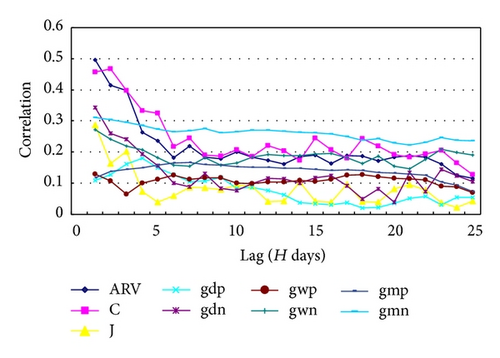
In Figure 1, ARV, C, J, gdp, gdn, gwp, gwn, gmp, and gmn, respectively, represents ARV_t, C_t, J_t, , , , , , and in Chinese stock market. Figure 1 shows, for the CSI 300 series studied in this paper, the lagged correlation function between the estimated daily integrated variance ARV_t+h with X_t as a function of h, with X_t being ARV_t itself, C_t, J_t, , , , , , and . Seeing from the correlation function between ARV_t and ARV_t+h (namely, the autocorrelation function of ARV_t), we can find that ARV_t in Chinese stock market has obvious long memory character. Thus, the past ARV_t has certain forecast effect on future ARV_t, which is in line with the conclusions of previous studies. In addition, from correlation functions between ARV_t+h and other 8 variables, we can find that all function values in future 25 phases are greater than 0, so all the past values of these variables contain some forecast information towards the future ARV_t in Chinese stock market. However, the correlation function value of J_t and to ARV_t+h is very small, which shows that these two variables have relatively weaker forecasting performance on the future ARV_t in Chinese stock market. Based on the above analyses, it can be seen that the capital gain overhang g_t in Chinese stock market carries with it provides more information of forecasting the future ARV_t. Therefore, we can roughly judge that introducing the momentum effect (capital gain overhang) in the HAR-ARV-CJ model can improve the model’s forecasting performance of the future ARV_t in Chinese stock market.

Details are in the caption following the image — **Figure 1**
Open in figure viewer PowerPoint

Lagged correlation function between ARV_t+h and X_t.

4.2. Parameter Estimation

To show the superiority of measuring volatility in Chinese stock market of the new model (HAR-CJ-M model) in this paper, we first estimate the parameters in the HAR-CJ-M model, and also to that of HAR-ARV and HAR-CJ model for comparisons (the HAR-ARV-CJ-M, HAR-ARV, and HAR-CJ models mentioned here and that followed are all logarithm forms, that is, model (22), model (14), and model (16).) As the HAR-type models mainly focus on different market participations of different frequency in daily, weekly, and monthly markets when considering the heterogeneous character of the market, this paper chooses three values for H (1, 5 and 22), namely, , , and represent, respectively, the ARV of future 1-day, 1-week, and 1-month in Chinese stock market. Standard OLS regression is consistent and normally distributed, but when multistep ahead forecast is considered, the presence of regressors, which overlap, makes the usual inference no longer appropriate. Therefore, we estimate above models by OLS with Newey-West covariance correction.

The estimation results of the HAR-CJ-M model are shown in Table 2. When forecasting future 1-day, 1-week, and 1-month ARV in Chinese stock market, coefficients of the daily continuous sample path variation , weekly continuous sample path variation , and monthly continuous sample path variation in phase t are all obviously positive at significance level of 1%. It shows that the past continuous sample path variation in Chinese stock market contains forecasting information on the future ARV. However, the coefficient of the daily discontinuous jump variation in phase t is only significant when forecasting the future 1-day ARV, while neither the coefficient of the weekly discontinuous jump variation nor that of the monthly discontinuous jump variation is significant. Therefore, the discontinuous jump variation in Chinese stock market is weak in forecasting the future ARV. For the newly added the momentum effect factor (capital gain overhang g_t) in the HAR-CJ model, except that the coefficient of the nonnegative part of daily capital gain overhang is not significant when forecasting the future 1-week and 1-month ARV, the rest of coefficients of g_t are all obviously positive at significance level of 10%. This shows that the information contained in the capital gain overhang g_t in Chinese stock market has good forecasting performance on the future ARV. In this paper, we consider CSI 300 as a stock portfolio, and then we can use the momentum effect to explain part of the estimation results of the HAR-CJ-M model. We know from Grinblatt and Han’s research that the momentum effect leads to the positive correlation between the previous gains and losses (which is expressed by the capital gain overhang g_t) of CSI 300 and current gains and losses, respectively; hence the momentum effect helps in the rise and fall of CSI 300 and adds to its volatility. Therefore, the nonnegative part of past capital gain overhang in Chinese stock market is positive correlation with the future ARV, and negative correlation with the negative part, and can help with the forecasting on the future ARV to some extent. We make further analysis on the capital gain overhang of different phases (daily, weekly, and monthly), the daily capital gain overhang can represent the behaving characters of short-term investors in phase t in Chinese stock market, and the reference price of short-term investors is the 5-day moving average . When the price in phase t is higher than (namely, ), the disposition effect suppresses further rise of the stock price; when the price in phase t is lower than (namely, ), the disposition effect suppresses further fall of the stock price, thereupon the stock price reflects insufficient information of phase t; thus the momentum effect emerges. After phase t, the market gradually begins to reflect the previous information, so the momentum effect helps in the rise and fall of the market and increases the market volatility. Hence, the nonnegative part of the daily capital gain overhang is positive correlation with the future ARV, and the negative part of capital gain overhang is negative correlation with the future ARV. We can see from Table 2 that the value of γ_gnd is obviously greater than that of γ_gpd, and γ_gpd is not significant when forecasting the future 1-week and 1-month volatility. It means that short-term investors in Chinese stock market hold different attitudes towards the same amount of gains and losses in previous phases. The influence of previous losses on short-term investors is obviously greater than that of gains, which may be caused by the loss aversion of short-term investors. Similarly, the momentum effect can be adopted to explain the forecasting performance of the weekly capital gain overhang and monthly capital gain overhang on the future ARV in Chinese stock market. Different from the daily capital gain overhang , coefficients of the nonnegative part and negative part of both the weekly capital gain overhang and monthly capital gain overhang are, approximately, showing that the medium-term and long-term investors in Chinese stock market are basically the same in their attitudes towards the same amount of gains and losses in previous phases, and their loss aversion is not obvious. This also reflects that medium-term and long-term investors are more rational than short-term ones.

Table 2. Results of parameter estimation for HAR-CJ-M model.

	H = 1 (1 day)		H = 5 (1 week)		H = 22 (1 month)
	Coefficient	Std. error	Coefficient	Std. error	Coefficient	Std. error
γ₀	−0.2543***	0.0556	−0.1941***	0.0751	−0.0818	0.1006
γ_cd	0.1749***	0.0408	0.1458***	0.0325	0.0861***	0.0293
γ_cw	0.3592***	0.0627	0.2585***	0.0712	0.0931	0.0735
γ_cm	0.1773***	0.0543	0.2125***	0.0764	0.2995***	0.0852
γ_jd	0.0649*	0.0385	0.0125	0.0268	0.0098	0.0182
γ_jw	−0.0160	0.0418	0.0122	0.0504	0.0741	0.0459
γ_jm	0.0676	0.0534	0.0704	0.0750	−0.0065	0.0814
γ_gpd	0.0812*	0.0448	0.0291	0.0443	0.0557	0.0399
γ_gnd	0.3335***	0.0472	0.1836***	0.0467	0.0820*	0.0447
γ_gpw	0.0878***	0.0306	0.1053***	0.0392	0.1512***	0.0512
γ_gnw	0.0512*	0.0312	0.0774*	0.0398	0.1350***	0.0447
γ_gpm	0.1128***	0.0248	0.2023***	0.0355	0.2062***	0.0473
γ_gnm	0.1108***	0.0227	0.1868***	0.0344	0.2070***	0.0455

Adj-R²	0.6224		0.6807		0.6270

The estimation results of the HAR-ARV and HAR-CJ models are shown in Tables 3 and 4, respectively. With analysis of the estimation results in Table 3, we find that coefficients of the daily ARV (), the weekly ARV (), and monthly ARV () in phase t are all positive at significance level of 1% when the model forecast the future 1-day, 1-week or 1-month ARV in Chinese stock market. This shows that ARV in Chinese stock market has strong long memory character, and the past volatility contains forecasting information of future volatility. Meanwhile, it also shows that the volatility in Chinese stock market is affected by the past different volatility components. Different volatility components are produced by investor behaviors with different holding terms (short-term, medium-term, and long-term). This result also proves the existence of heterogeneous investors in Chinese stock market, which is in line with the Heterogeneous Market Hypothesis. With analysis of the estimation results in Table 4, when forecasting the future 1-day, 1-week, and 1-month ARV in Chinese stock market, it can be seen from the significance level of coefficients of , , , , and that the continuous sample path variation has good forecasting performance on the future ARV, while the discontinuous jump variation component has weak forecasting performance on the future ARV. It is in line with the analysis conclusion from the HAR-CJ-M model.

Table 3. Estimation results of the HAR-ARV model.

	H = 1 (1 day)		H = 5 (1 week)		H = 22 (1 month)
	Coefficient	Std. error	Coefficient	Std. error	Coefficient	Std. error
α₀	0.0021	0.0317	0.1475***	0.0532	0.3474***	0.0708
α_d	0.3658***	0.0436	0.2469***	0.0423	0.1420***	0.0267
α_w	0.2082***	0.0626	0.2151***	0.0734	0.1813***	0.0618
α_m	0.3196***	0.0522	0.3830***	0.0693	0.3889***	0.0773

Adj-R²	0.5642		0.6088		0.5445

Table 4. Estimation results of the HAR-CJ model.

	H = 1 (1day)		H = 5 (1week)		H = 22 (1month)
	Coefficient	Std. error	Coefficient	Std. error	Coefficient	Std. error
β₀	0.1540***	0.0303	0.2986***	0.0490	0.4776***	0.0624
β_cd	0.3172***	0.0381	0.2438***	0.0345	0.1393***	0.0298
β_cw	0.3975***	0.0617	0.3352***	0.0683	0.2096***	0.0778
β_cm	0.1405**	0.0558	0.2079***	0.0784	0.3037***	0.0903
β_jd	0.1115***	0.0411	0.0416	0.0305	0.0256	0.0211
β_jw	−0.0446	0.0390	−0.0097	0.0570	0.0725	0.0545
β_jm	0.1402***	0.0529	0.1767**	0.0762	0.0994	0.0813

Adj-R²	0.5868		0.6297		0.5495

Comparing the adjusted coefficient of determination Adj-R² of the HAR-CJ-M, HAR-ARV, and HAR-CJ models, we find that Adj-R² of the HAR-CJ-M model is obviously greater than that of the HAR-CJ and HAR-ARV models. When the three models measure ARV at future 1-day, 1-week, and 1-month, Adj-R² of the HAR-CJ-M model is 0.0356, 0.0510, and 0.0775 higher than that of the HAR-CJ model, respectively, and 0.0582, 0.0719, and 0.0825 higher than that of HAR-ARV model respectively. This shows that the past capital gain overhang in Chinese stock market contains much information of forecasting the future ARV.

4.3. Robustness to Models

This paper adopts the method of Grinblatt and Han [17] to give explanation to the momentum effect, in this way, the choice of reference price in the capital gain overhang can make great influence on the study of the momentum effect. So the choice of reference price is crucial in this paper. In the empirical evidence above, we take the 5-day, 5-week (25 days), and 5-month (110 days) moving average as the reference price for those short-term, medium-term, and long-term investors in Chinese stock market, respectively. Here we will adopt the 10-day, 10-week (50 days), and 10-month (220 days) moving average of CSI 300 in Chinese stock market as the reference price to do the robustness tests to the result in Section 4.2. The evaluation result of the HAR-CJ-M model is shown in Table 5, most of the coefficients of the capital gain overhang are significant, showing that the past capital gain overhang in Chinese stock market is helpful in forecasting the future ARV to some extent. Moreover, Adj-R²of the HAR-CJ-M model which takes the 10-day, 10-week (50 days), and 10-month (220 days) moving average of CSI 300 in Chinese stock market as the reference price is obviously greater than that of the HAR-CJ and HAR-ARV models, which accords with the result in Section 4.2. However, its Adj-R² is smaller than that of the HAR-CJ-M model which takes the 5-day, 5-week (25 days), and 5-month (110 days) moving average as the reference price. This shows that the 5-day, 5-week (25 days), and 5-month (110 days) moving average affects more of the decision-making behaviors of those short-term, medium-term, and long-term investors in Chinese stock market. Therefore, adopting the 5-day, 5-week (25 days), and 5-month (110 days) moving average as the reference price to forecast the future ARV in Chinese stock market is more suitable.

Table 5. Estimation results of the HAR-CJ-M model.

	H = 1 (1 day)		H = 5 (1 week)		H = 22 (1 month)
	Coefficient	Std. error	Coefficient	Std. error	Coefficient	Std. error
γ₀	−0.2092***	0.0618	−0.2042**	0.0869	−0.0809	0.1243
γ_cd	0.2373***	0.0398	0.1743***	0.0333	0.0776***	0.0279
γ_cw	0.3039***	0.0643	0.2500***	0.0727	0.1334*	0.0755
γ_cm	0.2154***	0.0625	0.2263***	0.0854	0.3056***	0.0971
γ_jd	0.0891**	0.0394	0.0243	0.0277	0.0131	0.0178
γ_jw	−0.0404	0.0416	−0.0148	0.0501	0.0593	0.0486
γ_jm	0.0914*	0.0534	0.1217	0.0753	0.0248	0.0862
γ_gpd	0.0407	0.0369	0.0626	0.0453	0.0997**	0.0465
γ_gnd	0.1798***	0.0386	0.1338***	0.0428	0.1100**	0.0450
γ_gpw	0.1304***	0.0338	0.1676***	0.0454	0.1895***	0.0446
γ_gnw	0.0975*	0.0323	0.1421***	0.0433	0.1554***	0.0447
γ_gpm	0.0317	0.0258	0.0794**	0.0360	0.0778	0.0502
γ_gnm	0.0520**	0.0225	0.0929***	0.0309	0.1141**	0.0514

Adj-R²	0.6083		0.6677		0.6136

4.4. Forecasts

4.4.1. In-Sample Forecasts

Figures 2(a), 2(b), and 2(c) contain three in-sample forecast volatility sequences that are obtained by the HAR-CJ-M, HAR-ARV, and HAR-CJ models and a real volatility sequence. We adopt the loss functions to evaluate the volatility forecasting performance in Chinese stock market of the HAR-CJ-M, HAR-ARV, and HAR-CJ model. We mainly choose four loss functions to evaluation. They are the mean absolute error (MAE), mean absolute percentage error (MAPE), root mean squared error (RMSE), the heteroskedastic adjusted root mean squared error (HRMSE), and Theil coefficient. The smaller the values of these four loss functions are, the better the forecasting performance of the volatility models in future Chinese stock market is. The MAE, MAPE, RMSE, HRMSE and Theil coefficient for the in-sample forecasts from each of the three different models based on the data over the full sample period are reported in Table 6. Consider

()

where n is the number of samples predicted, ln (ARV_t+H) represents the true volatility, and

represents the forecast volatility.

Table 6. In-sample forecast statistics.

		MAE	MAPE	RMSE	HRMSE	Theil coefficient
H = 1	HAR-CJ-M	0.4352	1.6175	0.5641	0.6006	0.2228
	HAR-ARV	0.4674	1.9335	0.6083	0.6856	0.2425
	HAR-CJ	0.4530	1.5980	0.5913	0.6731	0.2346
H = 5	HAR-CJ-M	0.4437	4.3431	0.4037	0.4984	0.1469
	HAR-ARV	0.6015	5.3230	0.4518	0.9004	0.1660
	HAR-CJ	0.5514	4.4688	0.4368	0.7801	0.1609
H = 22	HAR-CJ-M	0.5700	4.7136	0.7002	0.5000	0.2579
	HAR-ARV	0.6514	6.5020	0.7896	0.5266	0.2897
	HAR-CJ	0.6174	5.9764	0.7466	0.5152	0.2742

In Table 6, we can find except that the MAPE of the HAR-CJ-M model is greater than that of HAR-CJ model when the model forecasts the 1-day ARV, the other MAE, MAPE, RMSE, HRMSE, and Theil coefficient of the HAR-CJ-M model are all smaller than those of the HAR-CJ model, and the MAE, MAPE, RMSE, HRMSE, and Theil coefficient of HAR-CJ model are all smaller than those of the HAR-ARV model. Therefore, the in-sample forecasting performance of the HAR-CJ-M model on future volatility in Chinese stock market is better than that of the HAR-CJ model, and the HAR-ARV-CJ model is better than that of the HAR-ARV model.

4.4.2. Out-of-Sample Forecasts

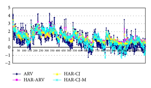
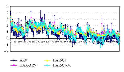
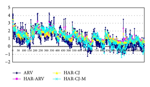
Compared with the in-sample forecasting performance, we are more concerned with the out-of-sample forecasting performance of the model, for the out-of-sample forecasting performance is more significant to the study of volatility in Chinese stock market. In order to make effective evaluation to the out-of-sample forecasting performance of the model, we divide the whole sample interval (from April 20, 2007 to April 20, 2012) into two parts the former part (from April 20, 2007 to May 31, 2011) has 1000 samples in all as the estimation intervals of the model; the latter part (from June 1, 2011 to April 20, 2012) has 199 samples in all as the forecasting intervals of the model. Figures 3(a), 3(b), and 3(c) contain three out-of-sample forecast volatility sequences that are obtained by the HAR-CJ-M, HAR-ARV, and HAR-ARV-CJ models and a real volatility sequence. In addition, the method of analyzing is the same with that of the Section 4.4.1, that is, using the loss functions to evaluate the out-of-sample forecasting performance of the model. The results are shown in Table 7.

Table 7. Out-of-sample Forecast Statistics.

		MAE	MAPE	RMSE	HRMSE	Theil coefficient
H = 1	HAR-CJ-M	0.4623	2.9898	0.6273	0.4201	0.5489
	HAR-ARV	0.5129	4.9047	0.6826	0.4501	0.9499
	HAR-CJ	0.4793	3.3916	0.6600	0.4338	0.5869
H = 5	HAR-CJ-M	0.4886	6.5385	0.6361	0.2202	0.5135
	HAR-ARV	0.5446	4.3915	0.7162	0.2932	0.6501
	HAR-CJ	0.4966	4.4688	0.6615	0.2484	0.5522
H = 22	HAR-CJ-M	0.5713	12.093	0.7168	0.4258	0.5137
	HAR-ARV	0.6524	12.249	0.8089	0.4852	0.6075
	HAR-CJ	0.6380	12.133	0.7652	0.4432	0.5245

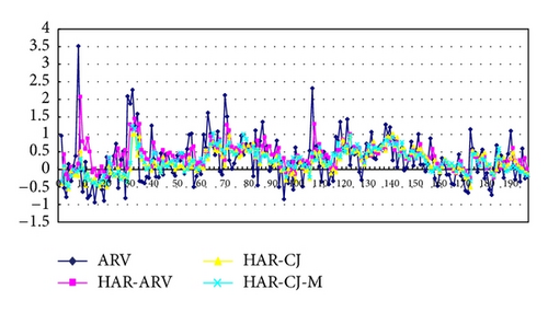
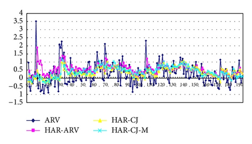
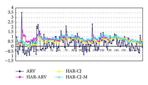
In Table 7, it can be found that except that the MAPE of HAR-CJ-M model is greater than that of HAR-ARV-CJ model, and that of HAR-ARV-CJ model greater than HAR-ARV model when forecasting the 1-week ARV, the rest values of MAE, MAPE, RMSE, HRMSE, and Theil coefficient of HAR-CJ-M model are all smaller than those of HAR-ARV-CJ model, and the MAE, MAPE, RMSE, HRMSE and Theil coefficient of HAR-ARV-CJ model are smaller than those of HAR-ARV model. Therefore, the HAR-CJ-M model has better out-of-sample forecasting performance on future performance in Chinese stock market than the HAR-ARV-CJ model, and the HAR-CJ model is better than the HAR-ARV model.

Combining the analyses in Sections 4.4.1 and 4.4.2, we can conclude that the forecasting performance of the above three volatility models of future volatility in Chinese stock market from the best to the weakest is in the following order: HAR-CJ-M model, HAR-ARV-CJ model, and then HAR-ARV model.

5. Conclusion

Considering the crucial role of the overnight return variance in volatility of the whole Chinese stock market, we convert RV into ARV and set up a HAR-CJ-M model on the basis of the HAR-CJ model and momentum effect. After that, we take the 5-minute high-frequency data of CSI 300 as samples for empirical evidence and estimate parameters on the HAR-CJ-M, HAR-ARV, and HAR-CJ models. Then we compare these three models of their forecasting performance of the future ARV in Chinese stock market by using the loss functions.

In the HAR-CJ-M model, most coefficients of the momentum effect (capital gain overhang) of different term limits (daily, weekly, and monthly) are significant, showing that the irrational behaviors of different kinds of investors in Chinese stock market help in forecasting the future volatility to some extent. In addition, from the estimate results of this model and the HAR-CJ model, we can see that the past continuous sample path variation in Chinese stock market can help with the forecast of future volatility, while the past discontinuous jump variation has very poor forecasting performance, which is in line with the conclusion of Wang et al. [13]. The estimate results of the HAR-ARV model show that the volatility of Chinese stock market can be influenced by the past different volatility components, and different volatility components are produced by behaviors of investors with different holding term limits (short-term, medium-term, and long-term). Thus, this result also proves the existence of the heterogeneous character of Chinese stock investors, which accords with the Heterogeneous Market Hypothesis. Besides, the comparative analysis of the above three models’ forecasting performance shows that the HAR-CJ-M model which has added the momentum effect forecasts much better than the other two models on the future volatility of Chinese stock market. Therefore, it shows that the irrational factors of investors do affect the volatility of Chinese stock market. Based on this, the volatility model which has taken the irrational factors of investors into consideration can forecast better on the volatility of Chinese stock market, and the HAR-CJ-M model is more favorable to the study of practical problems such as financial risk measuring, asset pricing, and financial derivatives pricing. Although the HAR-CJ-M model has good forecasting performance on future volatility in Chinese stock market, its Adj-R² is all smaller than 0.7 when it forecasts the future 1-day, 1-week, and 1-month volatility in Chinese stock market. So it is necessary to further improve the accuracy of the model’s forecasting volatility of Chinese stock market. Our work will be paid more consideration into irrational factors of investors on the basis of this paper so that further improve the forecasting accuracy of the model for the volatility in Chinese stock market.

Acknowledgments

The authors are extremely grateful to the Editor and the anonymous reviewers for their constructive and valuable comments, which have contributed much to the improvement of this paper. This work was supported in part by the Natural Science Foundation of China (nos.71171024, no. 11101053, No. 70921001), Hunan Province Graduate Research and Innovation Projects (CX2012B364), and the Scientific Research Funds of Hunan Provincial Science and Technology Department of China.

References

1 Engle R. F., Autoregressive conditional heteroscedasticity with estimates of the variance of United Kingdom inflation, Econometrica. (1982) 50, no. 4, 987–1007, https://doi.org/10.2307/1912773, MR666121, ZBL0491.62099.
10.2307/1912773
Web of Science® Google Scholar
2 Bollerslev T., Generalized autoregressive conditional heteroskedasticity, Journal of Econometrics. (1986) 31, no. 3, 307–327, https://doi.org/10.1016/0304-4076(86)90063-1, MR853051.
10.1016/0304-4076(86)90063-1
Web of Science® Google Scholar
3 Taylor S. J., Modeling Financial Time Series, 1986, John Wiley & Sons, Chichester, UK.
Google Scholar
4 Andersen T. G. and Bollerslev T., Answering the skeptics: yes, standard volatility models do provide accurate forecasts, International Economic Review. (1998) 39, no. 4, 885–905, 2-s2.0-0005880209.
10.2307/2527343
Web of Science® Google Scholar
5 Andersen T. G., Bollerslev T., Diebold F. X., and Ebens H., The distribution of realized stock return volatility, Journal of Financial Economics. (2001) 61, no. 1, 43–76, 2-s2.0-0035402387, https://doi.org/10.1016/S0304-405X(01)00055-1.
10.1016/S0304-405X(01)00055-1
Web of Science® Google Scholar
6 Koopman S. J., Jungbacker B., and Hol E., Forecasting daily variability of the S & P 100 stock index using historical, realised and implied volatility measurements, Journal of Empirical Finance. (2005) 12, no. 3, 445–475, 2-s2.0-19644389883, https://doi.org/10.1016/j.jempfin.2004.04.009.
10.1016/j.jempfin.2004.04.009
Google Scholar
7 Wei Y. and Yu N. T., The predicting model of the volatility of China’s stock market and its SPA test, Journal of Financial Research. (2007) 7, 138–150.
Google Scholar
8 Wei Y., Volatility forecasting models for CSI 300 index futures, Journal of Management Sciences in China. (2010) 2, 66–76.
Google Scholar
9 Corsi F., A simple approximate long-memory model of realized volatility, Journal of Financial Econometrics. (2009) 7, no. 2, 174–196, 2-s2.0-62849101579, https://doi.org/10.1093/jjfinec/nbp001.
10.1093/jjfinec/nbp001
Web of Science® Google Scholar
10 Müller U., Dacorogna M., Dav R., Pictet O., Olsen R., and Ward J., Fractals and intrinsic time-a challenge to econometricians, Proceedings of the 39th International AEA Conference on Real Time Econometrics, October 1993, Luxembourg.
Google Scholar
11 Zhang B., Zhong Y. J., and Tian J. F., Long memory-driven factors of volatility in Shanghai complex index based on high frequency data, Statistics & Information Forum. (2009) 24, no. 6, 21–26.
Google Scholar
12 Andersen T. G., Bollerslev T., and Diebold F. X., Roughing it up: including jump components in the measurement, modeling, and forecasting of return volatility, The Review of Economics and Statistics. (2007) 89, no. 4, 701–720, 2-s2.0-36448949838, https://doi.org/10.1162/rest.89.4.701.
10.1162/rest.89.4.701
Web of Science® Google Scholar
13 Wang C. F., Yao N., Fang Z. M., and Li Y., An empirical research on jump behavior of realized volatility in Chinese stock markets, Systems Engineering. (2008) 2, 1–6.
Google Scholar
14 Andersen T. G., Bollerslev T., and Huang X., A reduced form framework for modeling volatility of speculative prices based on realized variation measures, Journal of Econometrics. (2011) 160, no. 1, 176–189, https://doi.org/10.1016/j.jeconom.2010.03.029, MR2745876.
10.1016/j.jeconom.2010.03.029
Web of Science® Google Scholar
15 Zhang X. F. and Tian J. F., A new realized volatility model driven by heterogeneous finance market, The Journal of Quantitative & Technical Economics. (2011) 9, 140–153.
Google Scholar
16 Jegadeesh N. and Titman S., Returns to buying winners and selling losers: implication for stock market efficient, Journal of Finance. (1993) 48, no. 1, 65–91.
10.1111/j.1540-6261.1993.tb04702.x
Web of Science® Google Scholar
17 Grinblatt M. and Han B., Prospect theory, mental accounting, and momentum, Journal of Financial Economics. (2005) 78, no. 2, 311–339, 2-s2.0-27244437891, https://doi.org/10.1016/j.jfineco.2004.10.006.
10.1016/j.jfineco.2004.10.006
Web of Science® Google Scholar
18 Frazzini A., The disposition effect and underreaction to news, Journal of Finance. (2006) 61, no. 4, 2017–2046, 2-s2.0-33746832945, https://doi.org/10.1111/j.1540-6261.2006.00896.x.
10.1111/j.1540-6261.2006.00896.x
Web of Science® Google Scholar
19 Hansen P. R. and Lunde A., Consistent ranking of volatility models, Journal of Econometrics. (2006) 131, no. 1-2, 97–121, https://doi.org/10.1016/j.jeconom.2005.01.005, MR2275996.
10.1016/j.jeconom.2005.01.005
Web of Science® Google Scholar
20 Martens M., Measuring and forecasting S & P 500 index-futures volatility using high-frequency data, Journal of Futures Markets. (2002) 22, no. 6, 497–518, 2-s2.0-0036248776, https://doi.org/10.1002/fut.10016.
10.1002/fut.10016
Web of Science® Google Scholar
21 Barndorff-Nielsen O. E. and Shephard N., Power and bipower variation with stochastic volatility and jumps, Journal of Financial Econometrics. (2004) 2, no. 1, 1–37, 2-s2.0-30744467415, https://doi.org/10.1093/jjfinec/nbi022.
10.1093/jjfinec/nbh001
Google Scholar
22 Barndorff-Nielsen O. E. and Shephard N., Econometrics of testing for jumps in financial economics using bipower variation, Journal of Financial Econometrics. (2006) 4, no. 1, 1–30, 2-s2.0-30744467415, https://doi.org/10.1093/jjfinec/nbi022.
10.1093/jjfinec/nbi022
Google Scholar
23 Andersen T. G., Dobrev D., and Schaumburg E., Jump-robust volatility estimation using nearest neighbor truncation, Journal of Econometrics. (2012) 169, no. 1, 75–93, https://doi.org/10.1016/j.jeconom.2012.01.011, MR2935265.
10.1016/j.jeconom.2012.01.011
Web of Science® Google Scholar

Citing Literature

All articles

Measuring and Forecasting Volatility in Chinese Stock Market Using HAR-CJ-M Model

Abstract

1. Introduction