Volume 2013, Issue 1 139216
Research Article
Open Access

Analysis of Stochastic Delay Predator-Prey System with Impulsive Toxicant Input in Polluted Environments

Meng Liu

Corresponding Author

Meng Liu

School of Mathematical Science, Huaiyin Normal University, Huaian 223300, China hytc.edu.cn

Search for more papers by this author
First published: 10 October 2013
Academic Editor: Massimiliano Ferrara

Abstract

A stochastic delay predator-prey model in a polluted environment with impulsive toxicant input is proposed and studied. The thresholds between stability in time average and extinction of each population are obtained. Some recent results are extended and improved greatly. Several simulation figures are introduced to support the conclusions.

1. Introduction

Environmental pollution by industries, agriculture, and other human activities is one of the most important socio-ecological problems in the world today. Due to toxins in the environment, lots of species have gone extinct, and many are on the verge of extinction. Thus, controlling the environmental pollution and the conservation of biodiversity are the major focus areas of all the countries around the world. This motivates scholars to study the effects of toxins on populations and to find out a theoretical persistence-extinction threshold.

Recently, a lot of population models in a polluted environment have been proposed and investigated; here, we may mention, among many others, [123]. Particularly, Yang et al. [15] pointed out that in many cases toxicants should be emitted in regular pulses, for example, the use of pesticides and the pollution by heavy metals (see, e.g., [24]). Thus, they proposed the following two-species Lotka-Volterra predator-prey system in a polluted environment with impulsive toxicant input:
()
where all the parameters are positive constants and  Δf(t) = f(t+) − f(t),   Z+ = {1,2, …};   x1(t) and x2(t): the size of prey population and the predator population, respectively; ri0: the intrinsic growth rate of the ith population without toxicant; ri1: the ith population response to the pollutant present in the organism; Ci0(t): the concentration of toxicant in the ith organism; Ce(t): the concentration of toxicant in the environment; kCe(t): the organism’s net uptake of toxicant from the environment; gCi0(t) + mCi0(t): the egestion and depuration rates of the toxicant in the ith organism; hCe(t): the toxicant loss from the environment itself by volatilization and so on; γ: the period of the impulsive effect about the exogenous input of toxicant; b: the toxicant input amount at every time.

Yang et al. [15] showed that in the following Lemma holds.

Lemma 1. For system (1), define

()
  • (a)

    If r10 < r11K1/γ, then lim t→+xi(t) = 0, i = 1,2.

  • (b)

    If r10 > r11K1/γ and , then and x2(t) goes to extinction.

  • (c)

    If , then ,  i = 1,2.

Some interesting and important problems arise naturally.
  • (Q1) In the real world, the growth of species depends on various environmental factors, such as temperature, humidity and parasites and so forth. Therefore population models should be stochastic rather than deterministic (May [25]). Thus, what happens if model (1) is subject to stochastic noises?

  • (Q2) In addition, time delays occur in almost every situation. Kuang [26] has pointed out that ignoring time delays means ignoring reality. Therefore, what happens if model (1) takes time delays into account?

  • (Q3) Can we improve the results given in Lemma 1?

The aim of this paper is to study the above problems. Suppose that stochastic noises mainly affect the growth rates, with (see, e.g., [2739]), where is a white noise and is the intensity of the noise. Moreover, taking time delays into account, we obtain the following model:
()
with initial condition
()
where τi ≥ 0, τ = max {τ1, τ2}, ϕi(t) is continuous on [−τ, 0]. Our main result is the following theorem.

Theorem 2. For system (3), define

()
  • (i)

    If θ1 < r11K1/γ, then both x1 and x2 go to extinction almost surely (a.s.); that is, lim t→+xi(t) = 0  a.s.,   i = 1,2.

  • (ii)

    If θ1 > r11K1/γ and , then x2(t) goes to extinction and x1 is stable in time average a.s.; that is,

    ()

  • (iii)

    If , then both x1 and x2 are stable in time average a.s.

    ()

Remark 3. By comparing Lemma 1 with our Theorem 2, we can see that on the one hand, if α1 = α2 = 0 and τ1 = τ2 = 0, then θi = ri0, , i = 1,2, and our stochastic delay system (3) becomes model (1); on the other hand, our results in Theorem 2 improve that in Lemma 1. Lemma 1 shows that the superior limit is positive, while Theorem 2 reveals that the limit exists and gives the explicit form of the limit. The contribution of this paper is therefore clear.

2. Proof

For the sake of simplicity, we introduce some notations:
()

Lemma 4. For any given initial value , there is a unique global positive solution x(t) = (x1(t), x2(t)) T to the first two equations of system (3) a.s.

Proof. The proof is similar to Hung [29] by defining

()
and hence is omitted.

To begin with, let us consider the following subsystem of (3):
()

Lemma 5 (see [13], [15].)System (10) has a unique positive γ-periodic solution , and for each solution (C10(t), C20(t), Ce(t)) T of (10), , , and as t. Moreover, and for all t ≥ 0 if and , i = 1,2, where

()
for t ∈ (nγ, (n + 1)γ] and nZ+. In addition,
()

Lemma 6 (see [34].)Suppose that x(t) ∈ C[Ω × [0, +), R+].

  • (I) If there exist σ and positive constants σ0,  T such that

    ()

  • for tT, where Bi(t) are independent standard Brownian motions and βi are constants, 1 ≤ in, then one has the following: if σ ≥ 0, then 〈x〉 *σ/σ0 a.s.; if σ < 0, then lim t→+x(t) = 0  a.s.

  •   

    (II) If there exist positive constants σ0,  T and σ such that

    ()

  • for tT, then 〈x〉 *σ/σ0 a.s.

Now, let us consider the following auxiliary system:
()
with initial value .

Lemma 7. If , then the solution y(t) of system (15) obeys

()

Proof. By Lemma 5,

()
Then, for all  ε > 0, there exists T > 0 such that
()
An application of Itô’s formula to (15) yields
()
That is to say, we have shown that
()
()
When (18) is used in (20), we can see that for t > T,
()
()
Let ε be sufficiently small such that θ1r11K1/γr11ε > 0. Making use of (I) and (II) in Lemma 6 to (22) and (23), respectively, we have
()
It then follows from the arbitrariness of ε that
()
Substituting (17) and (25) into (20) and noting that lim t→+t−1B1(t) = 0, one can derive that
()
Employing (20) and (21) in the expression a21ln (y1(t)/y1(0)) + a11ln (y2(t)/y2(0)) yields
()
In view of (25), we get
()
By (17), (26), (27), and (28), for all  ε > 0, there exists T > 0 such that, for tT,
()
()
If , then we can choose ε sufficiently small such that . Then, by (29) and (I) in Lemma 6, we obtain lim t→+y2(t) = 0  a.s. If , then we can choose ε sufficiently small such that . An application of (I) and (II) in Lemma 6 to (29) and (30), respectively, makes one observe that
()
Therefore, using the arbitrariness of ε results in
()
This completes the proof.

We are now in the position to prove our main results.

Proof of Theorem 2. Applying Itô’s formula to (3) leads to

()
()

(i) It follows from (17) and (33) that

()
for sufficiently large t. Since θ1r11K1/λ < 0, then we can choose ε sufficiently small such that θ1r11K1/λ + ε < 0. Then, by (I) in Lemma 6,
()
When (36) is used in (34), one can see that
()
for sufficiently large t, where ε > 0 obeys −θ2 + ε < 0. In view of Lemma 6 again, lim t→+x2(t) = 0,  a.s.

(ii) By the stochastic comparison theorem [40], one can observe that

()
Note that θ1 > r11K1/γ and ; it then follows from Lemma 7 that lim t→+y2(t) = 0,  a.s. Making use of (38) gives lim t→+x2(t) = 0,  a.s. Thus, for all  ε > 0, there exists T > 0 such that, for tT,
()
Substituting the above inequalities into (33) and then using (18), we obtain
()
()
Let ε be sufficiently small such that θ1r11K1/γε > 0, and then, applying (I) and (II) in Lemma 6 to (40) and (41), respectively, one can see that
()
An application of the arbitrariness of ε gives
()

(iii) Clearly, implies θ1 > r11K1/γ, and then, by Lemma 7,

()
Thus, similar to the proof of (28), we get
()
Therefore, by (26), (28), and (38), we can observe that
()
()
Employing (33) and (34) in the expression a21ln (x1(t)/x1(0)) + a11ln (x2(t)/x2(0)) yields
()
When (18), (46) and (47), are used in (48), one can obtain
()
for sufficiently large t, where ε > 0 obeys . It then follows from (II) in Lemma 6 that
()
By virtue of the arbitrariness of ε, we can see that
()
Consequently, for every , there is T > 0 such that
()
Substituting the above inequality into (33) and then using (18) and (47), one can see that
()
for sufficiently large t. Since , and then, by Lemma 6 and the arbitrariness of ε, one can observe that
()
When this inequality, (18) and (47), are used in (34), we can see that
()
for sufficiently large t. Then, it follows from Lemma 6 and the arbitrariness of ε that
()
Substituting the above inequality and (18) into (33), we get
()
for sufficiently large t. By (II) in Lemma 6 and the arbitrariness of ε again, we obtain
()
Then, the required assertion follows from (51), (54), (56), and (58).

3. Numerical Simulations

Let us use the famous Milstein method (see, e.g., [41]) to illustrate the analytical results.
To begin with, we choose r10 = 0.85,   r20 = 0.05,   r11 = r21 = 1, a11 = 0.4,   a12 = 0.4, a21 = 0.3, a22 = 0.3, τ1 = 3, τ2 = 8, , ki = gi = mi = 0.1, i = 1,2, h = 0.5, b = 0.6, and γ = 12. Then,
()
By (c) in Lemma 1, the solution of model (1) obeys
()
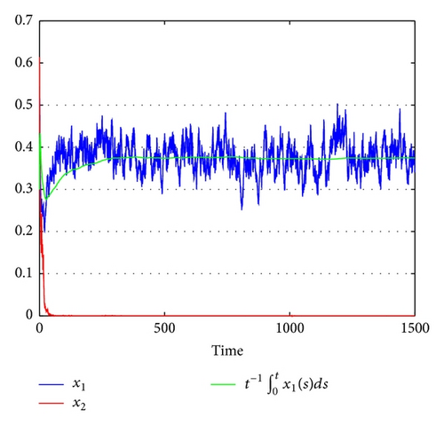
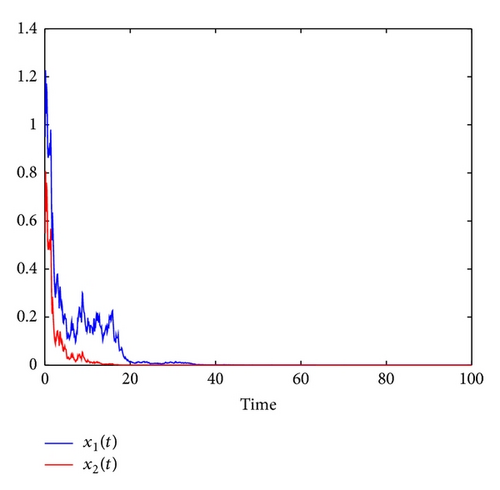
However, when the white noises are taken into account, the properties of the system may be changed greatly. In Figure 1, we let the coefficients be same with the above. The only difference between conditions of Figures 1(a), 1(b), and 1(c) is that the value of is different. In Figure 1(a), we choose . Therefore,
()
Then, by (i) in Theorem 2, both x1 and x2 are extinctive. Figure 1(a) confirms these. In Figure 1(b), we choose . That is to say θ1 = 0.2 > r11K1/γ = 0.05 and . It then follows from (ii) in Theorem 2 that x2 is extinctive and x1 is stable in time average:
()
See Figure 1(b). In Figure 1(c), we choose . Then, . In view of (iii) in Theorem 2, we can obtain that both x1 and x2 are stable in time average:
()
Figure 1(c) confirms these.
Details are in the caption following the image
Solutions of system (3) for r10 = 0.85, r20 = 0.05, r11 = r21 = 1, a11 = 0.4, a12 = 0.4, a21 = 0.3, a22 = 0.3, τ1 = 3, τ2 = 8, , ki = gi = mi = 0.1, i = 1,2, h = 0.5, b = 0.6, γ = 12, x1(0) = 0.9, x2(0) = 0.5, C0(0) = Ce(0) = 0.1, and step size Δt = 0.001. (a) is with ; (b) is with ; (c) is with .

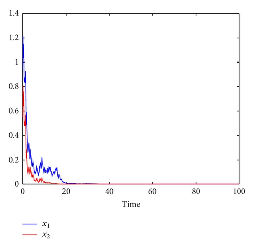
In Figure 2, we choose r10 = 0.85, r20 = 0.05, r11 = r21 = 1, a11 = 0.4, a12 = 0.4, a21 = 0.3, a22 = 0.3, τ1 = 3, τ2 = 8, , , ki = gi = mi = 0.1, i = 1,2, h = 0.5, and b = 0.6. The only difference between conditions of Figures 1(c) and 2 is that the value of γ is different. In Figure 2, we choose γ = 0.8. Then, θ1 = 0.65 < r11K1/γ = 0.75. It follows from (i) in Theorem 2 that both x1 and x2 are extinctive. Figure 2 confirms these. By comparing Figure 1(c) with Figure 2, one can see that the impulsive period γ plays a key role in determining the stability in time average and the extinction of the species.
Details are in the caption following the image
Solutions of system (3) for r10 = 0.85, r20 = 0.05, r11 = r21 = 1, a11 = 0.4, a12 = 0.4, a21 = 0.3, a22 = 0.3, τ1 = 3, τ2 = 8, , , ki = gi = mi = 0.1, i = 1,2, h = 0.5, b = 0.6, γ = 0.8, x1(0) = 0.9, x2(0) = 0.5, C0(0) = Ce(0) = 0.1, and step size Δt = 0.001.

4. Conclusions and Future Directions

This paper is concerned with stochastic delay predator-prey model in a polluted environment with impulsive toxicant input. For each species, the threshold between stability in time average and extinction is established. Some recent results are improved and extended. Our Theorem 2 reveals some interesting and important results.
  • (A)

    Firstly, time delay is harmless for stability in time average and extinction of the stochastic system (3).

  • (B)

    The white noise α1dB1(t) and α2dB2(t) can change the properties of the system greatly.

  • (C)

    The impulsive period γ plays an important role in determining the stability in time average and the extinction of the species.

Some interesting questions deserve further investigations. One may consider some more realistic but more complex systems, for example, stochastic delay model with Markov switching (see, e.g., [30, 32, 39]). It is also interesting to investigate what happens if aij is stochastic.

Acknowledgments

The author thanks the editor and reviewer for these valuable and important comments. This research is supported by NSFC of China (nos. 11301207, 11171081, 11301112 and 11171056), Natural Science Foundation of Jiangsu Province (No. BK20130411) and Natural Science Research Project of Ordinary Universities in Jiangsu Province (no. 13KJB110002).

      The full text of this article hosted at iucr.org is unavailable due to technical difficulties.