Global Attractivity of a Diffusive Nicholson′s Blowflies Equation with Multiple Delays
Abstract
The present paper considers a diffusive Nicholson′s blowflies model with multiple delays under a Neumann boundary condition. Delay independent conditions are derived for the global attractivity of the trivial equilibrium and the positive equilibrium, respectively. Two open problems concerning the stability of positive equilibrium and the occurrence of Hopf bifurcation are proposed.
1. Introduction
Luo and Liu [16] studied the global attractivity of the nonnegative equilibria of (3).
Though the global attractivity of the nonnegative equilibria of (2) has been studied by Yang and So [10] and Wang and Li [13, 17], they just gave some sufficient conditions. Furthermore, as far as we know, the stability for partial functional differential equations with several delays was investigated by few papers. Motivated by the above excellent works, in this paper, we consider the global attractivity of the nonnegative equilibria of the systems (4)–(6) and present some conditions which depend on coefficients of the systems (4)–(6). When n = 1, our results complement those in Yang and So [10] and Wang and Li [13].
It is not difficult to see that if , then (4) has a unique nonnegative equilibrium N0 ≡ 0 and if , then (4) has a unique positive equilibrium .
The rest of the paper is organized as follows. We give some lemmas and definitions in Section 2 and state and prove our main results in Section 3. In Section 4, several simulations are obtained to testify our results, and some unsolved problems are discussed.
2. Preliminaries
In this section, we will give some lemmas which can be proved by using the similar methods as those in Yang and So [10].
Lemma 1. (i) The solution N(t, x) of (4)–(6) satisfies N(t, x) ≥ 0 for .
(ii) If ψ(θ, x)≢ 0 on Dτ, then the solution N(t, x) of (4)–(6) satisfies N(t, x) > 0 for .
Next, we will introduce the concept of lower-upper solution due to Redlinger [18] as adapted to (4)–(6).
Definition 2. A lower-upper solution pair for (4)–(6) is a pair of suitably smooth function v and w such that
- (i)
v ≤ w in ,
- (ii)
v and w satisfy
()for all with , and - (iii)
v(θ, x) ≤ φ(θ, x) ≤ w(θ, x), (θ, x) ∈ Dτ.
The following lemma is a special case of Redlinger [19].
Lemma 3. Let (v, w) be a lower-upper solution pair for the initial boundary value problem (4)–(6). Then, there exists a unique regular solution N(t, x) of (4)–(6) such that v ≤ N ≤ w on .
The following lemma gives us boundedness of the solution N(t, x).
Lemma 4. (i) The solution N(t, x) of (4)-(6) satisfies
(ii) There exists a constant K = K(ψ) ≥ 0 such that N(t, x) ≤ K on .
Proof. Let w(t) be the solution of the following Cauchy problem:
Solving the equation, we have
Taking
By Lemma 3, there is a unique regular solution N(t, x) such that
Note that
Therefore, the formula (8) is correct, and there exists one K(ψ) > 0 such that for any t ∈ (−τ, ∞) and
So we complete Lemma 4.
3. Main Results and Proofs
Theorem 5. Assume that , then every solution N(t, x) of (4)–(6) tends to N0 = 0 (uniformly in x) as t → +∞.
Proof. By Lemma 4, without loss of generality, let for . Under the condition , we can get
Define m(t) and y(t) to be the solutions of the following two delay equations, respectively:
By using the similar methods to prove Lemma 4, we can get that
Because of N(t, x) < 1/a, for any , m(t) ≤ φ ≤ y(t) < 1/a, one can get
Therefore, from Definition 2, (m(t), y(t)) is a lower-upper pair of (4)-(5) with initial condition m(θ) ≤ ψ(θ, x) ≤ y(θ) on Dτ. Consequently, by Lemma 3, we have
By Theorem 1 of Luo and Liu [16], it follows from that the solutions m(t) and y(t) of (17) both satisfy
Hence, we complete the proof of Theorem 5.
Proof. Let f(x) = xe−ax, then the function f(x) is increasing on (0, (1/a)) and decreasing on ((1/a), +∞), f(1/a) = max x∈[0,∞)f(x), for . Let , then it is not difficult to verify that the function g(y) satisfies the following conditions:
-
(g1) the function g(y) is increasing on (0, (1/a)) and decreasing on ((1/a), +∞), ,
-
(g2) g(y) > δy for y ∈ (0, N*) and g(y) < δy for y ∈ (N*, +∞).
There are now two possible cases to consider.
Case 1 (N* < 1/a). In view of Lemma 4, we may also assume without loss of generality that every solution N(t, x) of (4)–(6) satisfies
Let , , and . By (23), we have
From Lemma 1(ii), let
Let I∞ = {1,2, …}. Now, we define two sequences {zk} and {yk} to satisfy, respectively,
We prove that {zk} and {yk} are monotonic and bounded. First of all, we prove that {zk} is monotonically increasing, and N* is the least upper bounded. Note (g1) and (g2), we have
By induction and direct computation, we have
Similarly, we have
Define v1(t) and w1(t) to be the solutions of the following differential equations, respectively:
It follows from (24) and (25) that z0 ≤ N(t, x) ≤ y0 for any . Consider (30), for any , we have
Therefore, from Definition 2, (v1(t), w1(t)) is a lower-upper pair of (4)-(5) with initial condition z0 ≤ N(t, x) ≤ y0 on . Consequently, by Lemma 3, we have
Note that w1(t) is monotonically decreasing for t ≥ 3τ and lim t→∞w1(t) = y1, while v1(t) is monotonically increasing for t ≥ 3τ and lim t→∞v1(t) = z1. Hence,
Define vn(t) and wn(t) to be the solutions of the following differential equations, respectively:
Repeating the above procedure, we have the following relation:
By (28) and (29), and taking limits on both sides of (35), we have
Case 2 (N* = y0). Similarly, let yk = N* and zk be the same as in the proof of Case 1; we can also get (35). Hence, the proof of Theorem 6 is complete.
Remark 7. Our main results are also valid when N does not depend on a spatial variable x ∈ Ω in (4).
4. Numerical Simulations and Discussion
In this section, we will give some numerical simulations to verify our main results in Section 3 and present several interesting phenomena by simulations that we cannot give a theoretical proof. We just consider the case n = 2 in (4).
4.1. Numerical Simulations
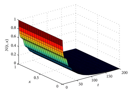
Different parameters will be used for simulations, and some data come from [20]. Figure 1 corresponds to the case with δ = 0.4, p1 = 0.1, p2 = 0.15, a = 0.1, τ1 = 12, and τ2 = 15, and under the above conditions, we have 0 < (p1 + p2)/δ = 0.625 < 1. We choose the initial condition ψ(θ, x) = 1, (θ, x)∈[−15,0]×[0,1], and the solution N(t, x) is decreasing and almost zero at time 160.

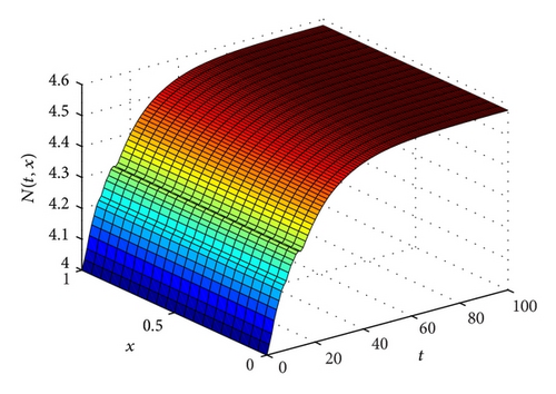
Figure 2 corresponds to the case with δ = 0.1, p1 = 0.1, p2 = 0.15, a = 0.2, τ1 = 12, and τ2 = 15, and under the above conditions, we have 1 < (p1 + p2)/δ = 2.5 < e and N* = 4.58145. Choose the initial condition ψ(θ, x) = 4 + sinθ, (θ, x)∈[−15,0]×[0,1]. From Figure 2, we can observe that the solution N(t, x) oscillates around 13 and 14 days; however, N(t, x) tends to N* as time t tends to 100 days. Therefore, Figures 1 and 2 support our main results (Theorems 5 and 6).

4.2. Discussion
In Section 3, we obtain two main results under the conditions and , which are independent of the delays τi, i = 1,2, …, n. A natural problem is what will happen when and the delays τi, i = 1,2, …, n are changed.
It is similar to Theorem 3 in Luo and Liu [16]; we present the following open problems.
Open Problem 1. If and aN*(eδτ − 1) ≤ 1, then every nontrivial solution N(t, x) of (4)–(6) satisfies
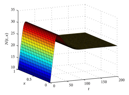
Figure 3 corresponds to the case with δ = 0.01, p1 = 0.5, p2 = 0.5, a = 0.2, τ1 = 12, τ2 = 15, and N* = 23.0259, and initial condition is ψ(θ, x) = 10 + sinθ, (θ, x)∈[−15,0]×[0,1]. Under the above conditions, we have (p1 + p2)/δ = 100 > e and aN*(eδτ − 1) = 0.745274 < 1. Sufficient conditions are dependent on coefficients and delay for the global attractivity of equilibria N*, and Figure 3 shows that the Open Problem 1 is right, but we cannot prove that.

From Figure 4, we have ((p1 + p2)/δ) = 5 > e and aN*(eδτ − 1) = 30.717 > 1. The condition is not satisfied, but N* is still globally attractive.

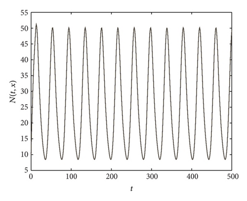
From Figure 5, we have ((p1 + p2)/δ) = 50 > e and aN*(eδτ − 1) = 13.6204 > 1. The condition is not satisfied, but the global attractivity N* is not true. Moreover, Figure 5 shows that there is a periodic solution, which is very interesting. We guess that the reason is that the system brings Hopf bifurcation as the parameters change. Therefore, we state the following open problem.

Acknowledgment
Project was supported by Hunan Provincial Natural Science Foundation of China (12jj4012) and Research Project of National University of Defense Technology (JC12-02-01).


