Spatial Cluster Analysis by the Adleman-Lipton DNA Computing Model and Flexible Grids
Abstract
Spatial cluster analysis is an important data-mining task. Typical techniques include CLARANS, density- and gravity-based clustering, and other algorithms based on traditional von Neumann’s computing architecture. The purpose of this paper is to propose a technique for spatial cluster analysis based on DNA computing and a grid technique. We will adopt the Adleman-Lipton model and then design a flexible grid algorithm. Examples are given to show the effect of the algorithm. The new clustering technique provides an alternative for traditional cluster analysis.
1. Introduction
Deoxyribonucleic acid computing, or DNA computing in short, has attracted strong interests and wide focus recently. It is inspired by the similarity between the way DNA stores and manipulates information with traditional Turing machine. Although DNA computing is in a sense similar to evolutionary computing, but the significant difference between them lies in the computing medium, biomolecules rather than transistor chips. It is this difference that makes DNA computing a promising field with ultimate goal of making DNA computers [1].
The essential work to reveal the ability of DNA in computing is by Adleman’s experiment (Adleman [2]), which demonstrated that the tools of laboratory molecular biology could be used to solve computation problems. Adleman also proves the huge information storage capacity of DNA which is contained in the sequence of nucleotide bases that hydrogen bonds in a complementary fashion to form double-stranded molecules from single-stranded oligonucleotides. Adleman’s work was later generalized by Lipton [3] to the satisfiability problem. Based on Adleman and Lipton’s research, a number of applications of DNA computing in solving combinatorially complex problems such as factorization, graph theory, control, and nanostructures have emerged [1]. There appeared also theoretical studies including DNA computers which are programmable, autonomous computing machines with hardware in biological molecules mode, see [4–7] for references.
Adleman and Lipton’s original works include a basic computing model, often referred to as the Adleman-Lipton model. Later generalizations include the sticker model, the splicing model, and the insertion deletion model [1]. However, most applications in this area are restricted to problems of combinatory types due to searching nature of DNA computing. It is a challenge how to design applications of optimization types.
Spatial cluster analysis is a traditional problem in knowledge discovery from databases [8]. It has wide applications since increasingly large amounts of data obtained from satellite images, X-ray crystallography, or other automatic equipment are stored in spatial databases. The most classical spatial clustering technique is due to Ng and Han [9] who developed a variant PAM algorithm called CLARANS, while new techniques are proposed continuously in the literature aiming to reduce the time complexity, or to fit for more complicated cluster shapes.
For example, Bouguila [10] proposed some model-based methods for unsupervised discrete feature selection. Wang et al. [11] developed techniques to detect clusters with irregular boundaries by a minimum spanning tree-based clustering algorithms. By using an efficient implementation of the cut and the cycle property of the minimum spanning trees, they obtain a performance better than O(N2). In another paper, Wang and Huang [12] developed a new density-based clustering framework by a level set approach. By a valley seeking method data points are grouped into corresponding clusters.
Although DNA computing and cluster analysis receive much attention and rapid development, there have appeared rare combination of these two important research areas. Up to the authors knowledge, the combination of DNA computing and cluster analysis is found in a few researches such as Bakar et al. [7].
Inspired by the research of Bakar et al. [7], this paper focuses on the joint study of DNA computing with cluster analysis. We propose a new grid-based clustering technique which can be solved by DNA computing. Different with other researches, this can reduce the searching space significantly. Finally we present two examples to show the details of our technique.
2. DNA Computing and Operations
2.1. DNA Structures
Macromolecules of nucleic acids are composed of nucleotide building blocks. In DNA, the nucleotides are the purines adenine (A), guanine (G), the pyrimidines thymine (T), and cytosine (C). Single-stranded DNA molecules, or oligonucleotides, are formed by connecting the nucleotides together with phosphodiester bonds. The single strands of DNA can form a double-stranded molecule when the nucleotides hydrogen bonds to their Watson-Crick complements, and (Figure 1).
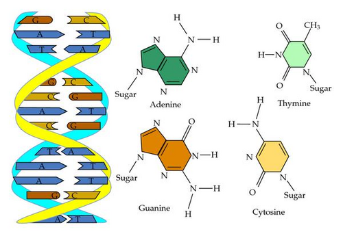
DNA stores information in nucleic acid and manipulates information via enzymes and interactions. A strand of DNA is encoded with four bases represented by the letters A, T, C, and G. Each strand has a 3′- and a 5′-end, and hence any single strand has a natural orientation. The cutting of certain strands of a DNA molecule is performed by the restriction enzymes. These enzymes catalyse the cutting operations at very specific DNA base sequences which are called recognition sites. Figure 2(a) shows a DNA molecule in which its four nucleotides in the left end and five in the right end are not paired with nucleotides from the opposite strand caused by cutting, or some other operations. In this case, the molecule is called to have sticky ends.


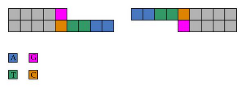
The effect is to cut the molecule into two pieces as shown in Figure 2(c).
There are over 100 different restriction enzymes, each of which cuts at its specific recognition site. A restriction enzyme cuts DNA into pieces with sticky ends. On the other hand, sticky ends will match and attach to other sticky ends of any other DNA that has been cut with the same enzyme. DNA ligase joins the matching sticky ends of the DNA pieces from different sources that have been cut by the same restriction enzyme.
2.2. DNA-Computing Models
There are several types of DNA-computing models among which the Adleman-Lipton model is the most traditional one. This model focuses on the hybridization between different DNA molecules as a basic step of computations. According to Adleman and Lipton’s original works [2, 3], this traditional DNA-computing strategy is based on enumerating all candidate solutions, and then using some selection process to choose the correct DNA. This technique requires that the size of the initial data pool increases exponentially with the number of variables in the calculation.
Apart from the Adleman-Lipton model, other DNA computing models appeared such as the sticker model, the splicing model. The Sticker model is based on a coding scheme called DNA complex. A DNA complex is a partially double DNA strand. Usually a double piece represents a bit with value one while a single-strand represents zero. Hence each complex is constructed by two single stranded DNA molecules referred to as memory strands and sticker strands. A memory strand contains n nonoverlapping substrands each of which is m bases long. Each sticker strand is m bases long and is complementary to exactly one of the n substrands in a memory strand.
The second model is the splicing model proposed by Tom [6] based on formal language theory. A splicing system S = (A, L, B, C) consists of a finite alphabet A, a finite set I of initial strings in A* (language over A), and finite sets B and C of triples (c, x, d) with c, d, x ∈ A*. Each such triple in B or C is called a pattern. For each such triple the string cxd is called a site, and the string x is called a crossing. Patterns in B are called left patterns, and patterns in C are called right patterns. The language L = L(S) generated by S consists of the strings in I and all strings that can be obtained by adjoining to Lucxfq and pexdv whenever ucsdv and pexfq are in L and (c, x, d) and (e, x, f) are patterns of the same hand. A language L is a splicing language if there exists a splicing system S for which L = L(S).
The next model is the k-armed model which is based on some more complicated molecule structures which have three-dimensional DNA architecture. In [13] the authors pointed out that it is natural to use the armed model to represent SAT problem in terms of contact network framework, and they gave theoretical solutions to this NP-complete problems. Like the splicing model, biological operations in the k-armed model include cleaving and connecting.
2.3. Operations of the Adleman-Lipton Model
The basic principle of DNA computing is to use the encoded information in the sequence of nucleotides and evolve them by breaking and making new bonds between them to reach the answer. The basic operations performed by enzymes are denaturing, replicating, merging, detecting, and so forth.
According to the DNA computing models proposed by Adleman [2] and Lipton [3], there are several basic DNA operations. One important operation is hybridization which is a main process in DNA computing to form all possibilities of solution strands in which the right answer lies. Hybridization is done by mixing strands in tubes with the help of some enzymes.
- (i)
Merge. m(N1, N2)≜N1 ∪ N2 = N.
- (ii)
Amplify. Duplicate (N1) = N.
- (iii)
Detect (N).
- (iv)
Separate or extract. N ← +(N, w), N ← −(N, w). Given a word w consisting of strings from Σ = {A, G, C, T} and a tube N, generate two tubes +(N, w) and −(N, w) which contain and does not contains the string w.
- (v)
Length separate. N ← (N, ≤n). Given a tube N and an integer n, generate a tube containing stands with length less or equal to n.
- (vi)
Position separate. N ← B(N1, w), N ← E(N1, w). Given a tube and word generate a tube with stands beginning (ending) with the word.
3. Grid-Based Clustering
The grid-based clustering uses a multiresolution grid structure, called cells, which contains the data objects and acts as operands of clustering performance. Traditional approaches include STRING WaveCluster, and CLIQUE [8]. The most common grids are regular hypercubic grid. This requires that the grid construction covers all the data space with the same precision. The second method uses flexible grids, that is, multiresolution grids with hypercubic or hyperrectangular cells having randomly oriented borders [14].
3.1. A Flexible Grid Definition
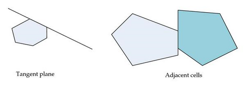
Suppose that the data set is Ω = {x1, …, xN} ⊂ Rn. It is bounded by a rectangle D0 in Rn. A grid is a undirected graph 𝒢 = (V, E) where each node of V is called a cell and is represented by a quad v = (D, c, p, σ), where D is a polyhedra, c is a center point of D, p = |ω∩D| is the number of points of Ω covered by the cell, and σ is the diameter of D. We will always assume that a cell is nontrivial; that is, D has interior points in Rn. For a cell v = (D, c, p, σ), its boundary is denoted by ∂D which is the set of hyperplane pieces bounding the polyhedra. If S ∈ ∂D and S is part of a hyperplane H, then H is called a tangent plane of the cell. Two nodes vi = (Di, ci, pi, σi), i = 1,2, are called adjacent if the two cells share a common tangent plane and D1∩D2 ≠ ∅. For two adjacent cells, define an edge between them. Hence, E = {uv : u and v are adjacent}. Figure 3 presents an illustration of tangent plane and adjacent cells.
To construct the graph 𝒢, we need two parameters p0 and σ0 indicating the minimum number of points to be considered, and the minimum diameter. Then the graph is constructed iteratively. We start with the first node v1 = (D0, c1, N, σ1), where D0 is the original rectangle, c0 is the center of D0. Then at each step, the cell containing dense points (controlled by a threshold value p0), or with larger diameter (controlled by threshold value σ0), is split into two subcells by a hyperplane. A cell is sparse if it contains less points than p0. It is called a small cell if its diameter is less than σ0. If we reach a sparse or small cell, then add this cell to the node set of the graph. This step continues until no more cell left to be split. The resulting graph is called a flexible grid. Algorithm 1 gives the algorithm for the graph construction process.
-
Algorithm 1: A flexible grid construction algorithm.
-
Inputs: Ω = {x1, x2, …, xN} dataset of N points in Rn, D: hyper-rectangle containing Ω, p0:
-
population threshold value, σ0: cell diameter threshold value
-
Outputs: V = {v1, v2, …}: set of vertices
-
Begin
-
V(1) = {v1 = (D0, c1, N, σ1)}. Let t = 1 and D1 = D0.
-
while V(t) ≠ ∅ do
-
for each v = (D, c, p, σ) ∈ V(t) do
-
Choose a cutting hyperplane L passing c. Cut the current cell v into two subcells v′, v′′.
-
For each v ∈ {v′, v′′} of the new cells, if pv < p0 or diam (Dv) < σ0, add this new cell v
-
to the node set V. Else add v to V(t + 1).
-
endfor
-
t = t + 1;
-
end
-
End
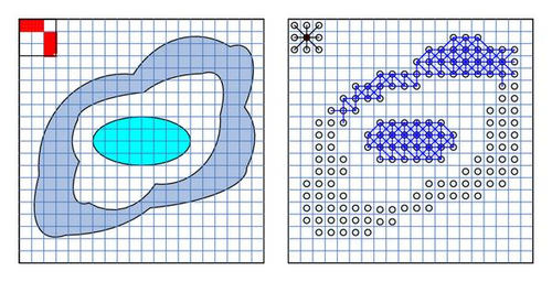
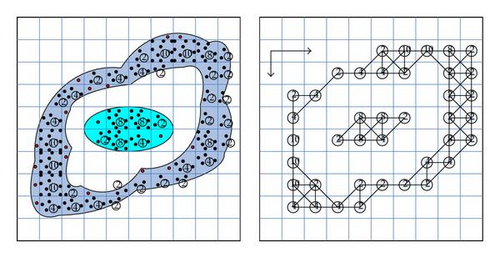
We present an example to show the data set and the flexible grid generated by the above algorithm (Figure 4).
3.2. Clustering Problems
When the graph is constructed, the clustering problem is converted into grouping nodes of the graph into clusters. Traditional techniques include the hierarchical clustering [8] For the purpose of this paper, we will give a different approach for this problem. First it should be noted that nodes corresponding to sparse areas are outliers. Therefore, in order to reduce computing complexity, we first remove all sparse graph nodes with corresponding edges. We still use 𝒢 = (V, E) to denote the resulting graph, where V is the set of vertices, and E the set of weighted edges. An example is shown in Figure 4 with part of its edges.
Then the clustering problem is a minimization of the energy functions. However, the optimization problem is hard to solve. We will present a variation in the following.
3.3. Path Clustering
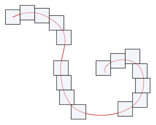
The first minimization of (3.4) is clustering for a fixed k, and the latter is clustering without fixing k. Path clustering is slightly different with distance-based clustering. The next example illustrates path clustering (Figure 5).
4. Clustering by DNA Computing
In this section we consider clustering of the graph 𝒢 = (V, E). We still use N to denote the number of nodes in V, and this will not cause any confusion. Suppose that the number of clusters is k which is a priori determined, or defined in the process of clustering. The problem is to partition the vertex set V into k clusters. Suppose that the original data set Ω is bounded by a constant M/2 > 0, that is, ∥x∥ ≤ M/2 for x ∈ Ω. Here we use the Euclidean distance for points in Rn and , where x = [a1, …, an]. Points in Ω are denoted by xi and Ω = {x1, …, xN}. A point in the data set Ω will be denoted by the lower case letter x.
For each point x ∈ Ω and a cluster C, define the distance between them as d(x, C) = min z∈Cd(c, z) where d(·, ·) is the Euclidean distance. If C1, C2 are two clusters, then define . Clearly these distances are bounded by the constant M. For u, v ∈ V define the dissimilarity measure as ρ(u, v) = ω(x, y)/M. Clearly these dissimilarity measures are in the interval [0,1].
Now we convert the dissimilarity measures into integers. First we need to define an acceptable error rate ε > 0. This means that we do not distinguish those measures where their difference is less than ε. Now we divide the interval [0,1] into I subintervals with equal width I−1 < ε. For z ∈ [0,1] let its corresponding integer be s(z) = [Iz] where operator [·] is the largest integer without exceeding it. Hence the dissimilarity measure lies in the set {1, …, I}.
Now we have converted the clustering problem to a permutation problem. That is, any permutation of the set {1,2, …, N, α, …, α} (the number of α’s is k − 1) is a candidate solution. The string with minimum length is the optimal solution.
4.1. DNA Coding for Data
The separator α is also coded with a single-strand seq (α) of the same length with that of points. This is done exactly as the data point coding except that we need to distinguish separators with data points.
4.2. Encoding Scheme
Now we need to put everything together for a candidate solution (4.3). First we design a code for an edge uv ∈ E with weight w. This is done by linking the last half part of seq (u), seq (w), and the first half of seq (v) as shown in Figure 6(a). We need two special edges called the left half-edge and the right half-edge. The left half edge is a linking of seq (u), seq (w), and the first half of seq (v). The right half edge is a linking of the first half of seq (u), seq (w), and seq (v).


Next we define coding for a centroid which is a complementary form of a separator α. First for two vertices u, v ∈ V, we define its similarity as . One should notice the difference with dissimilarity measure defined in the matrix W. Now we define the code of a centroid as a linking of the last half part of seq (u), seq (α), , and the first half of seq (v) as shown in Figure 6(c). Here u, v are two vertices in V.
4.3. DNA Program
Now we describe the biological operations for the clustering. First we put single strands in a tube T0 including complementary strands of all vertices, complementary strands of the separator α, and complementary strands of integers 1,2, …, I. These strands serve as splints. We also pour strands into T0 of all the left half-edges, right half-edges, strands of integers 1,2, …, I, all edges, and all centroids. Then hybridization and ligation can be executed. As a result, all combinations representing clustering schemes are obtained in the tube T0.
In order to select acceptable solutions among these combinations, we need to eliminate those strands which do not contain a separator α and those which do not contain all the vertices v1, …, vN. Finally, by counting the number of separators α as k of the strand with shortest length, we get the solution of the clustering problem. This final procedure can be implemented by direct observation to calculate the separator sequences by using special microscope such as atomic force microscope (AFM) to identify and calculate marking sequences [7].
The DNA program of biological operations is shown in Algorithm 2.
-
Algorithm 2: The DNA program.
-
Step and Procedure
-
(1) Input (T0).
-
All DNA sequences and complementary DNA sequences are placed in empty test tube T0.
-
(2) Amplify (T0).
-
Make all sequences in T0 mixed together and execute ligation process. After hybridization
-
process, all possible combinations of DNA sequences happen in T0.
-
(3) T1 ← +(T0, seq (α)).
-
Select only those DNA strands which include at least one separator α from T0 and keep them
-
into empty test tube T1.
-
(4) for i = 1 to N do {begin T1 ← +(T1, seq (vi)) end; }endfor; T2 ← T1.
-
Select all DNA strands that contain all the N vertices v1, …, vN in test tube T1. Put them in
-
empty test tube T2.
-
(5) Gel Electrophoresis.
-
Find the shortest DNA sequence in test tube T2. Put them in an empty tube T3. This is the
-
solution of clustering the problem.
-
(6) Count the number of separators α.
-
Amplify and count the number of clusters in tube T3.
-
END
5. Examples and Discussions
In this section, we present some examples to illustrate the performance of our algorithm. Then we will show that our technique will give clusters more naturally.
5.1. Example One
First we present an example with 20 points to be clustered that is discussed in [7]. First we construct a grid with interval 1 as shown in Figure 7. Then we take p0 = 1 as minimum points located in each grid. As a result, the induced graph is disconnected with 10 subgraphs. The final result shows four clusters with additional 6 outliers. This is different with result of [7] where they obtain four clusters with no outliers.
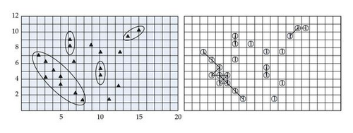
Now we change the grid into interval 2. Then we have only half the grids compared to grid with interval 1. We take p0 = 1 but we use another parameter ω0 = 1. This time we surprisingly obtain three clusters (Figure 8) with two outliers. This fact shows that the clustering method proposed here is sensitive to the construction of grids and parameters. Considering various definitions and measurements of clustering, this is not too surprising.
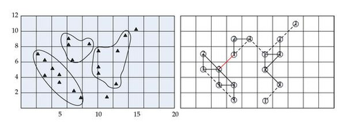
Now we construct a grid similar with Figure 8 but starting the first horizontal vertical lines not from coordinates (0,2) and (2,0). Identically, we can implement this case by moving the whole data set in the grid of Figure 8. With the same parameters as above, we obtain the third clustering result as shown in Figure 9. Now four clusters are generated without outliers. It is interesting to note that the three different grids induce one common cluster (left-bottom cluster). In fact, this common cluster is better organized than the other clusters. Hence we know that clustering is sensitive to the construction of grids especially for those bad clusters.
5.2. Example Two
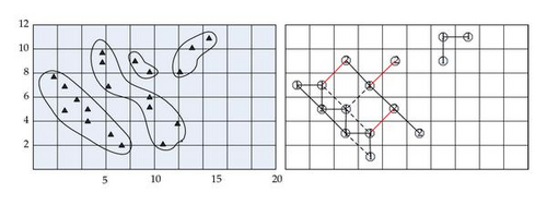
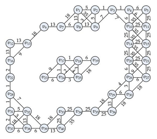
Now we consider another example as shown in Figure 10 with the data to be clustered and the graph constructed. For this example, we take p0 = 2. For adjacent cells, if they share a common edge, then we define their dissimilarity measure as 1. Otherwise if they share a common vertex, then define dissimilarity measure as 1.4. There are 40 nontrivial cells.
Here W1, W2, W3, and W4 are 20 × 20 matrices, and W is symmetric. The matrix W1, W3, W4 is shown in Table 1. The weighted graph is shown in Figure 11.
| 0 | 5 | 0 | 0 | 0 | 0 | 18 | 13 | 35 | 0 | 0 | 0 | 0 | 0 | 0 | 0 | 0 | 0 | 0 | 0 |
|---|---|---|---|---|---|---|---|---|---|---|---|---|---|---|---|---|---|---|---|
| 0 | 1 | 0 | 0 | 0 | 0 | 3 | 5 | 0 | 0 | 0 | 0 | 0 | 0 | 0 | 0 | 0 | 0 | 0 | |
| 0 | 1 | 0 | 0 | 0 | 0 | 7 | 7 | 0 | 0 | 0 | 0 | 0 | 0 | 0 | 0 | 0 | 0 | ||
| 0 | 6 | 0 | 0 | 0 | 0 | 6 | 6 | 0 | 0 | 0 | 0 | 0 | 0 | 0 | 0 | 0 | |||
| 0 | 0 | 0 | 0 | 0 | 35 | 25 | 0 | 0 | 0 | 0 | 0 | 0 | 0 | 0 | 0 | ||||
| 0 | 13 | 0 | 0 | 0 | 0 | 0 | 0 | 0 | 0 | 0 | 0 | 0 | 0 | 0 | |||||
| 0 | 6 | 0 | 0 | 0 | 0 | 0 | 0 | 0 | 0 | 0 | 0 | 0 | 0 | ||||||
| 0 | 13 | 0 | 0 | 0 | 0 | 0 | 0 | 0 | 0 | 0 | 0 | 0 | |||||||
| 0 | 0 | 0 | 0 | 0 | 0 | 0 | 0 | 0 | 0 | 0 | 0 | ||||||||
| 0 | 25 | 0 | 0 | 25 | 35 | 0 | 0 | 0 | 0 | 0 | |||||||||
| 0 | 0 | 0 | 35 | 25 | 0 | 0 | 0 | 0 | 0 | ||||||||||
| 0 | 13 | 0 | 0 | 13 | 0 | 0 | 0 | 0 | |||||||||||
| 0 | 0 | 0 | 9 | 0 | 0 | 0 | 0 | ||||||||||||
| 0 | 25 | 0 | 0 | 0 | 0 | 25 | |||||||||||||
| 0 | 0 | 0 | 0 | 0 | 35 | ||||||||||||||
| 0 | 0 | 0 | 0 | 0 | |||||||||||||||
| 0 | 1 | 0 | 0 | ||||||||||||||||
| 0 | 6 | 0 | |||||||||||||||||
| 0 | 0 | ||||||||||||||||||
| 0 | |||||||||||||||||||
| 0 | 0 | 0 | 0 | 0 | 0 | 0 | 0 | 0 | 0 | 0 | 0 | 0 | 35 | 25 | 0 | 0 | 0 | 0 | 25 |
| 0 | 0 | 0 | 0 | 0 | 0 | 0 | 0 | 0 | 0 | 0 | 0 | 0 | 0 | 2 | 0 | 0 | 0 | 0 | |
| 0 | 0 | 0 | 0 | 0 | 0 | 0 | 0 | 0 | 0 | 0 | 0 | 0 | 0 | 9 | 0 | 0 | 0 | ||
| 0 | 0 | 0 | 0 | 0 | 0 | 0 | 0 | 0 | 0 | 0 | 0 | 0 | 1 | 2 | 0 | 0 | |||
| 0 | 0 | 0 | 0 | 0 | 0 | 0 | 0 | 0 | 0 | 0 | 0 | 4 | 3 | 18 | 0 | ||||
| 0 | 0 | 0 | 0 | 0 | 0 | 0 | 0 | 0 | 0 | 0 | 0 | 0 | 0 | 6 | |||||
| 0 | 0 | 0 | 0 | 0 | 0 | 0 | 0 | 0 | 0 | 0 | 0 | 0 | 35 | ||||||
| 0 | 0 | 0 | 0 | 0 | 0 | 0 | 0 | 0 | 0 | 0 | 0 | 0 | |||||||
| 0 | 0 | 0 | 0 | 0 | 0 | 0 | 0 | 0 | 0 | 0 | 0 | ||||||||
| 0 | 0 | 0 | 0 | 0 | 0 | 0 | 0 | 0 | 0 | 0 | |||||||||
| 0 | 0 | 0 | 0 | 0 | 0 | 0 | 0 | 0 | 0 | ||||||||||
| 0 | 0 | 0 | 0 | 0 | 0 | 0 | 0 | 0 | |||||||||||
| 0 | 0 | 0 | 0 | 0 | 0 | 0 | 0 | ||||||||||||
| 0 | 0 | 0 | 0 | 0 | 0 | 0 | |||||||||||||
| 0 | 0 | 0 | 0 | 0 | 0 | ||||||||||||||
| 0 | 0 | 0 | 0 | 0 | |||||||||||||||
| 0 | 0 | 0 | 0 | ||||||||||||||||
| 0 | 0 | 0 | |||||||||||||||||
| 0 | 0 | ||||||||||||||||||
| 0 | |||||||||||||||||||
| 0 | 0 | 0 | 0 | 0 | 9 | 25 | 0 | 0 | 0 | 0 | 0 | 0 | 0 | 0 | 0 | 0 | 0 | 0 | 0 |
| 0 | 0 | 0 | 0 | 0 | 0 | 1 | 0 | 0 | 0 | 0 | 0 | 0 | 0 | 0 | 0 | 0 | 0 | 0 | |
| 0 | 6 | 0 | 0 | 0 | 0 | 0 | 0 | 0 | 0 | 0 | 0 | 0 | 0 | 0 | 0 | 0 | 0 | ||
| 0 | 3 | 0 | 0 | 0 | 0 | 0 | 0 | 0 | 0 | 0 | 0 | 0 | 0 | 0 | 0 | 0 | |||
| 0 | 0 | 0 | 0 | 0 | 0 | 0 | 0 | 0 | 0 | 0 | 0 | 0 | 0 | 0 | 0 | ||||
| 0 | 6 | 0 | 4 | 3 | 0 | 0 | 0 | 0 | 0 | 0 | 0 | 0 | 0 | 0 | |||||
| 0 | 0 | 0 | 18 | 0 | 0 | 0 | 0 | 0 | 0 | 0 | 0 | 0 | 0 | ||||||
| 0 | 0 | 0 | 1 | 7 | 0 | 0 | 0 | 0 | 0 | 0 | 0 | 0 | |||||||
| 0 | 6 | 0 | 0 | 0 | 0 | 18 | 13 | 0 | 0 | 0 | 0 | ||||||||
| 0 | 0 | 0 | 0 | 0 | 0 | 18 | 0 | 0 | 0 | 0 | |||||||||
| 0 | 5 | 0 | 0 | 0 | 0 | 2 | 3 | 0 | 0 | ||||||||||
| 0 | 0 | 0 | 0 | 0 | 18 | 13 | 18 | 0 | |||||||||||
| 0 | 25 | 0 | 0 | 0 | 0 | 18 | 25 | ||||||||||||
| 0 | 25 | 0 | 0 | 0 | 0 | 35 | |||||||||||||
| 0 | 25 | 0 | 0 | 0 | 0 | ||||||||||||||
| 0 | 0 | 0 | 0 | 0 | |||||||||||||||
| 0 | 6 | 0 | 0 | ||||||||||||||||
| 0 | 6 | 0 | |||||||||||||||||
| 0 | 13 | ||||||||||||||||||
| 0 |
6. Clustering of the Iris Data
In this section, we present another detailed examples to illustrate the encoding of the DNA-based clustering technique proposed in previous sections. The new example is the well-known Iris flower data set problem. The Iris flower data set is introduced by Sir Ronald Aylmer Fisher as an example of discriminant analysis [15]. The data set consists of 50 samples from each of three species of Iris flowers, that is, Iris setosa, Iris virginica, and Iris versicolor. Four features were measured from each sample, and they are the length and the width of sepal and petal [15, 16].
6.1. Grids and Graph of the Problem
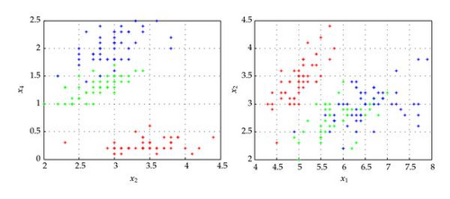
Then the cells can be denoted by 𝒟 = {Dpqrs∣20 × 16 × 30 × 15} with 144000 cells which is a huge number. Due to this reason, we choose x2x4 among the four dimensions as shown in the first image in Figure 12 as cluster feature variables. The second figure in the same image shows the other two dimensions x1x2 which is studied in Qu et al. [16].
| 0 | 67 | 236 | 67 | 118 | ||||||||
|---|---|---|---|---|---|---|---|---|---|---|---|---|
| 0 | 100 | 56 | 50 | 283 | ||||||||
| 0 | 177 | 500 | 500 | 707 | ||||||||
| 0 | 100 | 198 | ||||||||||
| 0 | 50 | 106 | 79 | 106 | ||||||||
| 0 | 133 | 99 | 99 | 250 | ||||||||
| 0 | ||||||||||||
| 0 | 125 | |||||||||||
| 0 | 125 | |||||||||||
| 0 | 395 | |||||||||||
| 0 | 999 | 999 | ||||||||||
| 0 | 999 | |||||||||||
| 0 | ||||||||||||
| 0 | ||||||||||||
| 0 | ||||||||||||
| 0 | ||||||||||||
| 530 | 0 | |||||||||||
| 158 | 0 | |||||||||||
| 0 | ||||||||||||
| 250 | 354 | 0 | ||||||||||
| 250 | 354 | 354 | 0 | |||||||||
| 250 | 0 | |||||||||||
| 354 | 354 | 0 | ||||||||||
| 0 | ||||||||||||
| 999 | 0 | |||||||||||
| 999 | 0 | |||||||||||
| 0 | 500 | |||||||||||
| 0 | 354 | |||||||||||
| 0 | 354 | 88 | ||||||||||
| 0 | 118 | 113 | ||||||||||
| 0 | 152 | |||||||||||
| 0 | 333 | 500 | 354 | |||||||||
| 0 | 157 | 143 | 200 | |||||||||
| 0 | 37 | 236 | 83 | 94 | ||||||||
| 0 | 16 | 39 | 22 | |||||||||
| 0 | 40 | |||||||||||
| 0 | 125 | |||||||||||
| 0 | 50 | |||||||||||
| 0 |
| 0 | 167 | 79 | 67 | 94 | ||||||
| 0 | 141 | 100 | 354 | 500 | ||||||
| 0 | 33 | 167 | ||||||||
| 0 | 40 | |||||||||
| 0 | 100 | 183 | ||||||||
| 0 | 500 | 707 | 500 | |||||||
| 0 | 999 | 999 | ||||||||
| 0 | 999 | |||||||||
| 0 | 999 | |||||||||
| 0 | ||||||||||
| 0 |
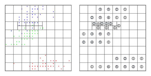
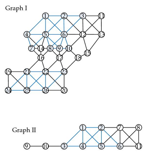
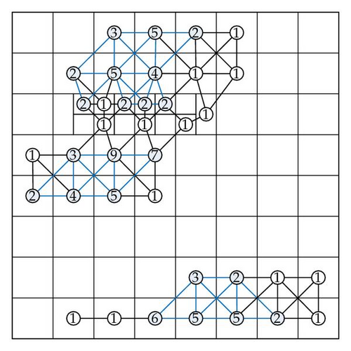
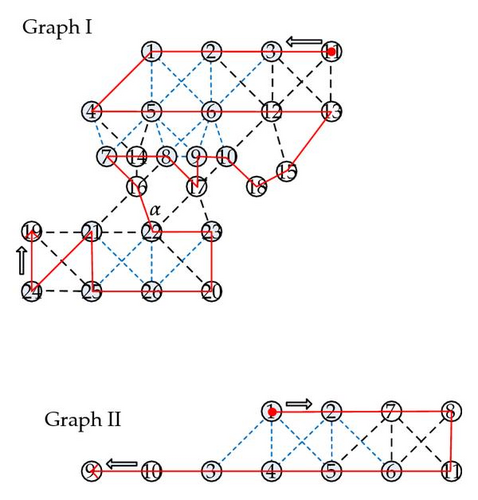
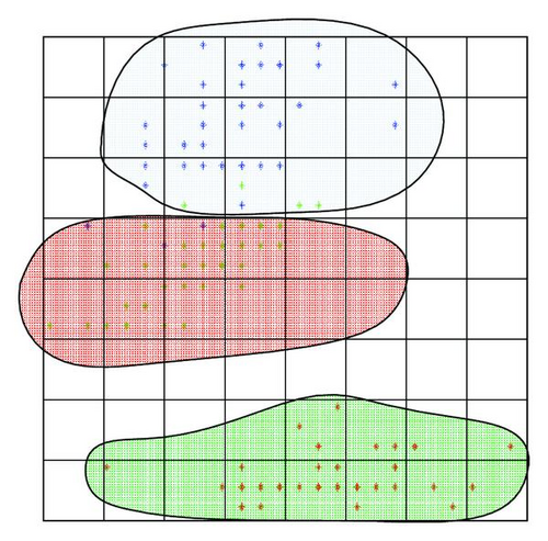
The detailed encoding scheme is shown in the Appendix. The final clustering result is shown in Figure 15(b). The number of points which is not correctly clustered is 7. Clearly this is much better than other methods such as CEPSO of [16] where the error number is more than 20.
6.2. Discussions
Now we present some discussions about the time and computational costs of the proposed technique in this section. According to Algorithms 1 and 2, the computational costs consist of two main procedures, that is, the grid construction and biological operations, and we will show that the complexity is roughly linear.
Next we analyze the complexity of DNA program as proposed in Algorithm 2. It is clear that the DNA program consists of three searching procedures. Step 3 selects those strands which contain at least one marker α which is a O(1) operation. Step 4 checks if we get a sequence containing all the vertices with a complexity of O(Nv), where Nv is the number of vertices and Nv ≤ N. The final Step 6 counts the number of α′s and splits the sequence into clusters. For the shortest sequence which contains all the vertices, the maximum number of markers α is Nv. Hence the total DNA complexity of the program is O(N) which is linear.
Finally we make some comments about experiments. By Adleman [2] and Păun et al. [1], when we design a DNA program for solving the problem, a test tube (as taken in the laboratory) is considered a multiset of words (finite strings) over the alphabet {A, C, G, T} with basic operations proposed as in [1, 2]. These basic operations are standard and biologically implementable.
However, when we want to simulate the algorithm with personal computers, there will appear some tricky complexity that lay behind the biological operations. Again we analyze the steps in Algorithm 2. First we consider Step 2, and we only consider generating sequences containing each vertex exactly once. The time complexity here will be . By examining other steps, we find the total time is O(2N).
7. Conclusion
In this paper we presented a new DNA-based technique for spatial cluster analysis. Two examples are given to show the effect of our algorithm. We do not need the number of clusters in advance. By a flexible grid method we can reduce the size of searching space significantly. This is different with other DNA-based applications in that they enumerate all solutions which will produce a large search space. This is especially useful for large database even through DNA computing that has large parallel ability. Also by changing the grid and corresponding parameters, we can get various clusters.
Finally we will point out that nonconvex clusters can be easily obtained by the technique of this paper. Comparing to research in [7] where only convex clusters can be generated, this is useful for complex database to be clustered. Up to the authors knowledge, this is, the first research in cluster analysis by DNA computing for nonconvex clusters. It provides an alternative solution for this traditional knowledge-engineering problem, which is not a combinatorial in nature. Comparing the many applications of DNA computing mainly in combinatorial problems, this is still interesting.
Acknowledgments
Research is supported by the Natural Science Foundation of China (no. 61170038, 60873058), the Natural Science Foundation of Shandong Province (no. ZR2011FM001), the Shandong Soft Science Major Project (no. 2010RKMA2005). The authors are indebted to the referee for important suggestions and the supplement of Section 6 and Appendix of the Iris Data Set Problem. We are also indebted to Dr. Qi Feng and Dr. Xue Jie for help in the design of DNA coding.
Appendix
DNA Encoding of the Iris Data
In this appendix, we present a DNA-coding scheme for the Iris data problem. By Tables 2 and 3 the weight values range from 16 to 999. Therefore, we need a maximum length of 999 mer to code the weights.
First we present one coding scheme for vertices of Subgraph I.
VERTEX CODING: 1. GGCCCATT GTCGACGA 2. AAGCATCC GAACGTCT 3. ATTTAGTA ACTGTCAT 4. CCACTAGG CATTTACT 5. TAACTGAA TAGCCTAA 6. CCCATCCT GACTGCAT 7. GATGTGCT CGTAGCCT 8. AACCCTTA CGTGCATC 9. ATGCCCAA CATATAGG 10. TATTTAGT TGAAGCAT 11. TTCAGGAG GTGCACTA 12. CGTTTAGC CACCTTAG 13. TGTATACA CTTTATGT 14. CAACCATA GCCGCCGT 15. TCCCCGTC ATACCTTG 16. TAGGTATG ACTCGGCG 17. AGAAATCG GCCGCAAT 18. GAGCGACT TCCTGGGT 19. CAATCATT TGCGGAGT 20. GCCGTGAT ACCCTCAG 21. AATGCACA GAGTTTAA 22. TAGACTGT GTAAATCG 23. TCTACCGC CGTCCTTG 24. AATGAACA TTAGTGGC 25. TCTGCATA CGCCCCGT 26. AGCGTTGT GTCCTTCT
Since the edge coding of vjvi is similar to those of vivj, we next only present coding for one edge between each two vertices as follows.
EDGE CODING: 1-2: CAGCTCGT GGCCCAACGCCCATTTCGTACCACGAGAACCCAAATAACGGAGCATAGAAGGGCATCTTACTTGGAG TTGCTAGC 1-4: CAGCTCGT AGCTACACGAGCTTCCGTATCGCTGTGTCGAATGGTGGGCCTTCTGTGGGAGTTAGGGGG CCGCTCAGACCCAGAATCGACCTGTTTATGCTGCCAGCTGTCAATGAATCTTAGAGTGTG AACGACATATCCTGTCGATTGTAG ATTGTTATCCTTGAAGAGATATACTTCGGCTTAGGC CTAGTTCGAAGGATCAAAACTACGCGTCAAAATCGGTCGCCGTTTATACCCCGTCC GGTGATCC 1-5: TTGCTAGC AACGCGCGGCCACCCTTAACTACCCAGTACCCACATCTCCTCTGGCATGTTGGG AAACTCGGGCTAT ATTGACTT 1-6: TTGCTAGT TACAAGAAAGCATTAGACCACAAATATCACGCGATTAAATCAATGGCTTAA AATCGCTGATTCATCGGTTAACAGACAGCGCTAGGTTACCGTGATACCGTAGCACTCGATCTTAGTC TCCTAGGA
2-3: GTTGCAGA AAACTTGAAGAAGCGTCAACGAGTCGGACCTTGGCACTGCTGGCGAGATCGCCGGACAAAATATGCATGTGCCCCCTACTTAAGGTAATCCGATTAGAGC TAAATCAT 2-5: GTTGCAGA CCACAGGAGATATGATATATCCTCGGCCACTGAGCCCTAGGCAACCCTGGTCTAAT ATTGACTT 2-6: GTTGCAGA GTAACCGCGAGCCCTAACGCTTACTCTTTGACGGGAGTCACGAACTGACG TCCTAGGA 2-12: GTTGCAGA GGCACTTTGA GATGTCGGTG AAACTGTCCT CCGATCTCAA CACTAGTGTG GAGTCTTCAC ATCACAATGG AACTCATACG GATAAGTCAG TCTGCCATGC CACAGGTAAA ATATGAGGCG AGGGCAG CTC TGGGCCTTTG TATCAGCCAG GTTCTATTGT TTCAGGGCCC TGGTTAGGCT GCAATCAAAT ACCCATAGTA TTTCTGAGCA CAATTCCAAA TGACGCCCAA ACAGACGTGG ATAAATTGGT ATGAAGTCTA TGACCGTTAA ACGGAGTTAC TTC GCAAATCG
3-6: TGACAGTA GTTTGGACAA TGCGAACTGC GAGGTATTCA GTTAGCAGGG TACCGACAGA ATATGTCCAG AAGCTT TGTT GGTCTAAAAA GTCACGGCCA ATTTGCTAGC GCGGGCTGTT ATACGCTCAA GATGGGCACC AGATGATATC CTCATCATTC GGCCGCAAGT GACTCTTCGA TTATACT TCCTAGGA 3-11: TGACAGTA GTCCAGGAAC CCCTTATTTT TTTGAAAGTT AACGACCGTT CTACCCGACG TTAGGGCTGA CGCCTTCCGT ATACCAACAG CAAGATTACG TGATGACGGA CCAAATATA G CTCGTTGCCA CAAGGGTACA ACTAGGCTTC GACAATGTAG AGGAACGCAA CGGGTCTGTG TCCTTCACAA ACCTACCTTT GGGAGGGTAG TGCTTGTTTT TATATCTTTC TATGAGCCAG AGAGTCGATG GCCTGATAAG GCTGCCATCG GCTAATTGGG TACTTCGGCG CTCCCGAATA GCCCAATTGT GTCAGCGAGA TACGGCCCTT GTGTTCAGCA TTGCCCTGTG ACAATTCATT GTACGACCGA CGCCCATCTA TGGGTGCGGG GGTGGTTTAA AGAATTCTAG GTGCTACCTG CGACTCACCA CCGCTGTTAT GACGGGGATA GTCGATACTA AAACTACCAT CATATTCATG CTCCGGAAGA GCCGGCCAGT ATAGGTATTC AAGTCCTC 3-12: TGACAGTA CTCAACTACG TTTAATTTAT GCGAAGCGAG TGATTAACCG AAGCGAAGGG TAGTACGGCT TCTACCGCCA GAACACGTAG ACAGCGTGG G AAAGCGATAG TTGACAGCTA AGTCGGTTGA GGCTGCACCC TGATGAACT C GTAATACATA GCTCAAGCTT CCATTGGTGG ATTCTTTACC GTAGTACGAC TCACCCACAG GAGTCGACAC TGTTGGCTTC ACTTCATCTA TCCCAGGGCT TTCCCGTTAG CAAGGCATTA TTAGACAGGG TATTGCCGGA CTAGCTAGCC TTAGCTATAA CAGGAAATAA TGCTGATTGG ACTGAACAGC GATGTGATTC CTCCAATAGC ATATATCCAT CGCCGAGTAT TCTTCGGTTG TTCGCGCATA CTTCCTAGGA ATACCGCCGA TTATGAATTC GCCCCAGGGA GAGTCCGTTC CGACCCATGA ATGATTTCAC CGGTCGCTGC GCTCGGTTCG TCATCTTGTG GCGAAAGGTC GCAAATCG 3-13: TGACAGTA AAGAAGCTGG CCACATTCGT CACCTAGCAT TGATTGGCGA TGTCGGTGAG GGAAATTGCC GCGGTACCAA GGCAGAACTT GCGGAGTCCG GTGAAGTATG GAACGCGGAA CACGAGCCGT AGCTAGTTTG ATGCTTTAAA AGCTTGAGAA ACAATACAAC CTGCCTGAAC CACGCTGCAG CAAGACGCGA GGCGCATTTA ATGGCGAGGT AACCAAGTAT GGTCCCCACC AGCTAACGAG ATTAGCCGAC AGAGCATTTC TTTGATGCAA CGATTAACGC GCTGGTCGCA ATGGTCCCAA GGGCGAGGGA AGCCCGGTTA TCAATGAAGG CCATTATGGG TAATCCCATA GACCAGGCTT GGTCAGAACC CTATCCTAGT AAGTCGGACG TTGGACGTTG CAAGAGTGCG AAACATGTCC GCATAGCGTT TGTAAGAACT ATCGAGGAAC TACCTTTGTC GATTGTCTAG AACATGCCCA TGAAGAGAGC ACAGACATGC CAACCCCAAA TTATGTAGGA AGGGTACGGT TCTAAGGTAT AGTTTTGAGG TTGTTCTTTT CGTCTACAGA AAAGATCCCC TCCGGGAGTA TAGTGCAAAA TCCATGGAAG AGCCCACAAA AGTCAGAAAT AGACTAATAT TCCATGTTAT CAATCAAGTT AATGCTTCAA CAAACCCTGA GCGTGCGCGA AGAAAAGTAG AGATTTA ACATATGT
4-5: GTAAATGA GAGAGGATTC CTGAGCTGTT CAGGCGGCGA GGCATCTAGG TGGTGCGGCA AAGAGATCTT CTTGTGTCCC ATCCCGCCCC TACCACTTAG ACCAAGACGA ATTGACTT 4-7: GTAAATGA TAGTGTGCTA GACATCTGGC CGCCGGCGCC AGCTCGTGGA TGCTCATAAG GCTTAACTTG ACGTCTTAGG AAGAAACTCA AGCCCAATCG CATTCTTCTT CACTGCAACA CGCGGTTGTT ACCGGCCTTT GAGTATCTTT TACTTCGCTT TAGGCCCACC TGCAGTAACC ATCGCTGTCA GAAT TAGCTG AACTTTTG CTACACGA 4-14: GTAAATGA TGCGGGTGTC TAAGAAATTT GCATGAATAA GTGCTGACTA AGTTATACCG AAAAAGTCTT GCGGGACGCA GGTTGCTGTC TCGTATCTCT GAGAGCTCGT GTCCGTTCGG CCGGGACGAT AGGATGCCCC CGACAATGAA CATGATCTTC GACCCACAAC GTACAAGACC CGAGCTAACA CTGCTCTAGT CATCCACGTA TTATTATTAC TACCACTAGC CAACGTGCAT CCCGCGTTGT AGTACGCAGG CTGTTTCACG ATGGCGATTT CCAACGGAAA GTTCTAACTT GACAGCGTAC CACTAAAGGA CGGCCAGGCA TGGGCATCGC AGTTTTGAGT ATTCACTCCG TGCACAACCG GACCTGACGT ACGTGAGGAC GAGGTCACCG GAACTAGACT CTATCCTCCG CGGGCACGAA CTATTGACTT CAAACGTACG GACACCTATC TTAATAGAGG ATTTGACGCA TACTCGCTAG CTGCCGGTTG CCTCGGCGGC GTTGGTAT
5-6: CCGGGTAA CGCGAATCGC GGGTAGTTCG TATCGTTGGA TGACTGCACT GCACATTTGC TCCTAGGA 5-7: CCGGG TAA ATGTCAATTC GGTAAGGACG TGGTGACATT GATGCATCTG CTCAGTGTGC CATATTCGTG CTCACTTCTT GCGCTATCTT TCGAGGGGTG TCACACACCT CTCAAG CTACACGA 5-8: CCGGGTAA GTCGCCCAGC TATCTGCCGC AGACAGGCAT ATAA CGGAAG GTATGGTGCC GTGCAGAGCT TTTGCGCAAT ACGCATGCA TTGGGAAT 5-9: CCGGGTAA GGCTCAGGCA CAACTGAAGA TTGACACACG TATAGCCAGC CGACCAACTA ATCACCACCG CGTGGGCTGT CTCGATTTTG CCCACTATTT GCCGGGTAGA ACGCGT TACGGGTT 5-14: CCGGGTAA TTTCTAGCGG GCCGCCATCT TACTGAGTAG ACAAGGAGGG CATTCTGAAC TTTACTTCAC TATCGAAGCG AGCGCCGCGG GCTGACAGCG ACAGTACACA TAAACGTAGT ACGTATATTC CACCACAATG CCTTGCCACC GTCACCGCGA GTCTAGAC GTTGGTAT
6-8: GGGTAGGA TGTACCCTCG CGAGGGCGCC AATTGCTAAG TACAATAACC CCACTGCTAG GCTATACACG ACGATCTAGC GTTCCAGTCG ACTCGCCCAG CTCACGATAA TGTGTACGCA ACAACGCCGC TGTCGAGCTC CAT TTGGGAAT 6-9: GGGTAGGA GCGCAAGACT TGATGAGTGA TCGTCCGTTC TGCCCGTGGA GATGCTGAAG CTCATACAGT ATGGCGCGCG ACAATCACTA TGCGGTGAAG TGTGGCCCC TACGGGTT 6-10: GGGTAGGA GTGGCCGGCT CCGCCAATCA GTCCACACGT TGATGCCTCG GGACGACTCT CGCGTAGAAG AGTATGTACT GGGACCCAAA AAGCTTGAGA GGATTTCGA ATAAATCA 6-12: GGGTAGGA AAGGAGAGCT CGGGGGGGAT GTTTATGAAG AAATGCAGTC AATACACTCT AACATCCTAC CCGAACAATC ATGATTAAAC GTAGTAGTTT ATCCTATAAT TCGCTCCGCC CTTGCCCCAG AAGCGATCAC CACCCACTAC AGTATACTGG GCTAACATAC GACGATTAAG TACCTTGTGC TAACCTCAAT TTCGCTACGC TCGTTGGGCT TATACCTACT AAAGCGAGGT CTACCACCTA CCCTAAAAAA GCAAATCG
7-14: GCATCGGA AGTAAATCAC GCCTTCATCT GAAGGCGAGT CGACCTACTT TCAGGTCGCT TTAGAATGCT ATATGAGATG ACGGAGGCAT TGGTTAAGTA CAACCTGACC AGCAACAACG AGTGGAACGG AGAGCGCGTA CAACTATATG TCACCTCATC TAAAAGAGCT TACGAGTTAC TAATGTACGG TGGGGAAACG GCTGAGTCGC CCCTCCGGTT GCTCCCGGGT AGAAGCCGGA GACGAGCACC GTCCACAGGG GTTGGTAT 7-16: GCATCGGA TGAGCCAGGG ACTGAAACGG TACCACCCAG TCGTGTGTTC TGGTATCTTG GGGCCGCCCT TATCGCAGCG ATGTCTCCAA GAAGGTCGTC AAAAGCAGAT GGAAG TTGAT GCATTCTCTG GCCGTAATGT ATGTAGGATA ACCCCTTAGT TCCAAACTGC AATCACCCAT TGATAGTTCC ACATGTCCTG GAATTAAAAA GGACCCTTAC ATCCTTAGCT TATGAGGTGC AGAATCCTTC TCTGGCGGCT ATGTAGTAAG GTCACGAACG TAGGTAGAGA CAAATCCGAG TTGATTCGCC ACACGTTGGC CGAGGCTCCG AGAAGGGGAC TTCAGACTGT TCTGGTTACC GCTG ATCCATAC
8-9: GCACGTAG GAATGAGCTT AAACTAATCA GTAAGGACCA GTCGGGGAAA CTCTAGCCCA TTGACCACCA GTTATTCTCG TCGGGTCGAG AGGCTCACAG ATAATTTAGA TACCGAGAAG CGAGTCTTAG GGGAA TACGGGTT 8-14: GTATAT CC CGGTACGATC AGAGACCCTC ACGCAGCAAC ATATAACAAT GCGGAAAATC TCGTGTCTCA AATGCGTACT ATTCATATCT GTTGAACACT ACTAGGCCGA ACGCAATGTT GTCAGGCCAA GCCACCGGCT ATAGGGATTT ATTTTACCCT CTTAGGCAG G ATTAAATAGG GGCCAACCAG TTGCTGGGCC TGGGTATATG TAATGCCTAA CCATAAACAG GAGGGAACCT GGGTTCAGCC ACACCATGCA GTCCACAGGG 8-16: GTATATCC GGAGAAGCGT GGCACCCTTG GGGGTAACTC TACATTCACC CAGGAGG GCC TCTCCGCTTT CAACTGGGCA ATCTAACATG TGTCCACCGT GTACCGGTAG CGCTACTGCC CGCTTCAAGA TGTAAGCGAG TACGCGTCAT CTGTTAGCGA TGAGCGATTC TAGCGGGACG AGAACAATAG TAGAGTCAAA CGGCTTGGAG CTAGAC AGCT TGTTTCTAAA CAACACTTAT CATTGCAACG GTGGGGGTAA GATATTCTTT AATGGACTCG CTAATATATG GGCCTGTTTA TGAGGACGCG GAACGTAAAT CCACCAAGGT CCGCCGAGTC ACATTCTTGC CTATCGTAAG CACT ATCCATAC 8-17: GTATATCC ACCTCGATGG ATTTCTGGTC TACCCAGGCA ATCGTTGATT CCCCAATGGC AACTCCAGTA GGGTGTTACC AATTCGACAC CTCGCAGATC ACACTGGCAC GGTGAGGCTC TCCGGCCGAT GATGGCAAAT CGGGTAATTC AGATGGGTAC AATTTGTTGG AGAAAATCGT GGCGCTTTGC TTCGACACCT CGGGATCGGC AAATCCAGTA GCGTGTATGC TTCGCATCCA GCGATGTAAC CATCCTTGAT TAGACGCAAA AGAAGATCAT GGACCGGTGC GGCGGGGATA CAATCGGTGT CTGGTGTCGA CCGACTGGTC CACCATCCCC CGGTGAGGGT ACGCGGTTGA TGAA TCTTTAGC
9-10: GTATATCC TGGGAGCTGA AACGAAGTCG ACACACTCAG CTCACCGCTA AGCTAGAGGG GGAAGTACCT TTGTATGATT CGGCTTGTCA GACTATCGAC CAGGGCTAGG ATACTGACGG TGCAGATCAG GTAGC ATAAATCA 9-17: GTATATCC GTACACAGCA GCGAGTCACA GACTCACCCC CACCCCAAAA GCATCGTGAT CTGTTGCCGA CTTGCGTTTA GCGCGTAAAG TTTTTACTTA GTATCTTACT CTCATGTAGC GTTATAGATA GACAATTCAT AGATCAGTAC TACAACGGCC CAGTTCT TGC AGCGGATTGC CTATTAAATT CGGACTTGTG AGATTTGATG ACCAAGTTAT AAAGGGTTCG TATTTGCAAT TCGCTGGTCT ACACCAAGCG TCTTTAGC
10-12: TCCTAGGA AATGTCCGTT CGGCAGGTTC TACGTTTAAT AGGTACGTCG GGTGATTTCA CTATCCGCGC TCACCCTAGC CATATCGATC TCACATCGAT CCGGTTAACT CGTTGCCCGT GCGGGAGGCT GCCGTTTCGG TAGGGTAGCA CTTTG AGGAA GAAGCAGACC GAACACTGAG TGTCGAGACC CATAGCTGAA TTAAAGCGAG CTTAGGGTAG GTGACAGCTG CGG GCCAATT TGGCAGCGTC GGACTGAATG ACATGGAACC GGCCTGAATC TGCGTGATTA TGAAGCTATC GCTTCTGGTT TCTCAAAACA AACTCTCAGA TGTGTTGCAC CCACAGGTCG TCCTTGGTCC CGAATCCAGC CTCATTCTTG GGATCGACTT AGAGGTCCAA AGCTT GCAAATCG 10-17: TCCTAGGA CCCAACTTAC ATAGGGATCA GAGTAACTTC ACCTGCTACT CTAGAGCTGT CAGGTACGCC CACTCACGTG AAGCACACCA GTTTACTCGT CTGAACGTTC GACGAGATAT TCGCCGGTAT AGATCGCGCC CTTTGATTTC TGTGCTCCCA AAAAGGATTT AGGTGTCAGA ACTGGTACTC CCGTAACGTT GGCTTTTAAG AGAGGTGCGG CTGTTCGGGA CCGTTCGTCG TGTCGCTCCA GGGTTCCTGG GTCGACATTC AGGGAGAAGC AAACAAAA CG TGGAAAAATG AAATCGCATG ACTTGCATGT TACTTATTTG CGGGACGAGA TTTTAAGGAA ATTGGTACCT CTAG TCTTTAGC 10-18: TCCTAGGA GATTACACCA CACGTACACA TAGCTTCCCA GATCCCTCAG GTCAGCTAAA TGACGCCCCC ACAAGACGGC TACGCTTACC ACCAATCGTA TCCGCGTGCA GTCCAGATGC GGCCCACACA GGCATCCAGA AACTAATTTG ACGGTTCTAC CACGACTGTC GAAAATTGCG ACGCCCAATT AGAACAATAC CGTAGACCGC GCGTTCTTGT CTAATTCTGT TTCCTCCGGA AATTCCATAC CGTTGGATAC TCCGCCGTTA AAGGGGTATG CTTCCGAACC AACAAAGGTA GATAAACGCG ACACCACGGT CTATTATACA TCCCCTGGCA ACCCCGGGCA CATCGCTCGT TTGA CTCGCTGA
11-12: CACGTGAT TAATATACAA AGACAACACT GGCATTCCAA GTTCAGTTCG GTCAACAATC CTAGATGGGG CGAG TTCATG ACGTGGAAGC CCATCAACAG CTGCACTTCG GGCAAATATG GTGCCCAAGG CTAGTCGCAC ATTACGACGA GAG AGGCACT GCCCTAGACC CAGGCACAGG CGAAGGAAAG CGCTCTGCCG GCGACCATAT ATAAATGACG GCTTAAGGTG GAATGACATA AAGCCGTCCC CCCAATCGGC TTATATGCAA GAGTACTGGC ATCAATCCTT TAGAGGCGTG TGGGACTGGC CGGTAAAATG GCATTTAGCC GAACTGACTA CCGCACCAGA AATGACTAGT CTTCAGTAAT CGTTTTCTTT ATCACAGGAC GTTCCTCTGG GCAGATTTGT CACGGTCCGC GACGCGCACT TCTGGTATAA TACTATGATA TTGGAAACAA CATGCCAGCC TCTACGCGCA CTTGGGCAAA CAAGGCTTAG GTCCAGATGA TTTCTCTCCA CGAGCACACC TGCCGTAAAT GAGAGATGCG TTTAGGAGTC GCACCTATAG GTCCTCTGCC GCACGAGAGT GTTTATTCCT CGCTCTGATT TCGAAATATT TCACAAATGT TCTAAGCTGC TTATGCTTCG TGATTTGACC CCCGTTGGTT AGCAGAATCT GCAGTCAATG AAGCTATTCC TCCATTCACC TGCAAAGTAA ACAGCGGGGT GATTCAGGGA TGCAAGTCGA TGGCCTAGTA ATGTGAGGTT TGATAAGTCA ATACTTAT CG GAGTATCATT ATTGCTTTTT GACCCCTTGG GCGGACAAGA ATCTACAACG ACGAACCGCA AGATAACGTT TAACTTACAT TGTTCACGTG CGCGGCCGGC AAAATATACG CGAGAAAGTC AGCTGTGTTG GGCAACCGGC CAAGGACTTG GACGCACCTC ATCGCAGCTT CGCACGTAAT TGGAGCGACT GTCAACTCAA TAGGTGCCCG TAACTCTGC GCAAATCG 11-13: CACGTGAT TGTATCTCGC ACACCGTTTA ACGTCTACCT TAGAACCCCC TGCTTTGCAT CATTTGTCTG AATGGCGGGC GCGATTGGGA GTTCGTGTTA TATAATTGCA GTCTGGCAAT AGAGATTTCG CGCAAGAAGG TACAGGCGCC CGACGCCCGC ACGCCCTCAC ATACCTTCTC TGTAATAGCA ACTGTCGCTC CGGAGCTCGG GATTGTACCC ACATGGTTGT GGTCTCTATG GCGGGGAAGA GAACATGACC TTTGACCTGT GTCCCGTAGC ATCTTGGCGT TCCTACTTGA GTGGATATTG ACCGAATTAA GACATACAGG TAATCTCGGC CGTTTGGAGC GCAATCCGCC GCTTACATTA TCAAAAATGA ATGCCCGGTA CCACATATTC GTCCCAGGGT CTTCTAGACC CCGTCCTGTG TATAACCGAA CCTCAGAACC AAGACCGCCT ACTACTGACA ATCCTGCGCC CAGAGCATCC CTAAAAGTGG TATTCTAAGG ACGCCGCGCT TTACGATTAG CGCTCATCGT TGTATTTAGT TTAAAATACT CTTAAGCGGT TGATGCGTAG GCCGCAATGG TTTCGCAAAG GCGTGGCACT GAGCTGCTGA ATAGTTGGGA GAGGCAAA GT GGAATTTCTG TTCCAAGCGC CAGGAGACCG CCAATGGAGC TTTCATTCCC AATAGGGACT TGATAATAGT CGGCGGCATA GAACGCTGGA TACAGCCATA TCGCCTGGCC TCCAGCCAGA AATCGTGCGC CAGTAGTTAG GCAACTCACG TTCGAAGAAT TGGACCTCTA GTGTGGCTGA AAGCTCGGCG CCACCAACAT GCAATTACTC TGCCCATATG CAGTCCGCCA TTGGCCCTCA ATATACCCAA GACAAGGGGA CGGAGATGAA CTCCACTGGT CGGCCACGTT CGAGGGGGGG CATTGCCGTG TGGCATCCGA TGGGTTCGCT TCTACCCTCG AGTGTTTACC CAACGCTGTA CTGGGGTTC ACATATGT
12-13: GTGGAATC AGGACCGCAC GGTCATTTGT TATTGTAACA CCTTGACAGG CGGCAACGGC TCGCCGGCAA GATACGCGAA GAGGAAATGG CGATTGAGGA TCTCAATTCA CTGGCCCCGA CTCCAGTTAC TGCCTCGATT TAGCTATGTT GCGAACTACA CGCGCTAGAG CAGCGTAGAT ACAGCTGACT CCCCTAAGCT GTTCCCGCGA AGCGTTATAG CGAATTTATA GC TCGGGCAT GGTGGATGGA CACCGCCCGG CTGACGCGTG CCAGGCCATG CAAGTCAGGC TTCTTGTTTG AGAACTAAAT AGCATCACAC CAAAGCTAAA CGGTCGGTGG GGTGGTCGCA TGTGCCTAGT CCTTCATGAA TGGATTCAGG CTATTTCAAG AGTTCCCGCG CACGAGGTCG CGATGTATAG GGGTTAGCAC CCATCACACG GAATCGGTGT TCTGACTACT GGAACGGTCG CCAGATATTC GTTGTACCGT TGATAACGCT ACCGTAATCA CCATTACCCG CACCACTACG ACAGGGGTTG GTTTTGCTCC CAGGTTTGTC CGGGGCGTCT GCTAATAGCG GCCTGGCAGT TGTCTAGTTA CTAGTAGCAT GGATACGTTT GGAGTTACGC GGCGTTAAGC TTTATTGGTC GTGGGCTCAA CATCGGTACC ACTGCGGCCC CACCAGGCGC CGTATAGCCG TGGGGGGATG AGGATTCTGC ACTACTGTAG TCCGACAGGC AGTGCGGAGG AATAGGATGA AGGGCGACCC GAGTTCGTCA AAATCCGCAC ACTATCAACT GTCCCCCGTC CCTTGCTACG GTGGAGGGGG TAATTCATCC CTGAGAGCAT AAGCAGTCAG TCAGGC TCGG GCCGGATATC GCATCGATGT ATTCCGCATT CTTGCTTCGC GGGGTGTCTG AAACATCTTG CGCCCCCAGC GACAGAACAT TATTCAAGTG GAAGCGGGCT CCAACCAGAA AGCAAACGGA ACGAAGGGCC AGCTATAGG ACATATGT 12-15: GTGGAATC ATACTAAGCA CCCTAGTTTA AAGAGTACCG CCGAAAACAT TGTTGAGGAT ACACTGCGAA TGCTGATTGA GACGGGAACC TGCGACATAC GGAACCAAGG GATCTCTATT AAAGCCGCTC GCTACTGACT AGATCCCGTA GATGTTACGC GACCTTAACT CGCTGATAGG GGATTCGCCG TGGGCGTTGT ACCACTGCGC CGACTTCTCT GCCGGCGCCG CCTCGGGTAA GTAACGGTTA GTAAGTGCAG TTGGTTTGGG CCGCATTGAG TGAGGTGCCT GCATGGTTTG ACTCTCATAT GCCTTGGGAG GACAAATTGA TCCCAGCAGA ACCAGATTTG TAGGATGATA GTTTGATAAA CACGTGAACA CTCCTCTATA AGTGCGCTGA GGGTGTCAAC AGACTTGTAT TAGGACCGGG GGCACACATC CGTTCATATG GCGTGGACCT AGCCCGAGGT TTTAGGTTAG TTACCCAACT AAACGCCTCA CATCTGATGA TACTTACGCA TTGCCTGACG AGTTGCGAGT TCTAGGCTAA AATAAAGATG TCGACAGTCG GTGGGATAAC ACTTTGGTGT GAGCGGATAT ATCAGAATGG CGGGACCATC TGGGATAAGC CCTCATGTTG GGACCTGGGC TGTCGAGGCC ACCTGCATGA ACTGCAAGTT TGACTACGTA GGCATTTGCC GCCCGTTTGA ACCAAACCGG CACTTACTAC TTGCGAAAAA AAACGAGTCC GAACCCAGCA TCGATCCGTT GCTACGGTCG AGTACTCAAT AATGGCGCTA AAATAGGTAC CGGCATCGTA GCCCCCTCGG TTAGCAATTC TGCAGTAATT ATAATATGGC AATTGAGGTT GAACACTTGC TATGCGGACC TTTACGAAGT TATGGCAGCG TGCGGGTCAG CTATTTTGGT AATCGCCCGC TGGTGTCTGA CCGCTACACA AACCGAATAC CGCACAATAC ACTGCCACAG CACTACTATC AGACTAAGA AGGGGCAG
13-15: GAAATACA CCGCGTTCGC CTGTGCGTAA GTCTAACAAG GCCCCGCGAA CAAACTATAT CCAGAAGATA GGTTCCCAGC GTCTGCTAAC GAATGTGTTT TATTGACATA CCAGGCAAGA GCTACTCCCC CTCAGGCCTA TTGGGGTAAC GATGATTCGC CATTAGGCAC CCGATGACTA TCGTAGACGC ACACCGTCGT TCGTCTACTA GGACAGTTTT AAGATGCTCC TTGGTACCAA TTGTGCAATG GGCTGAATCT ACACTTCCTG ATCATGGACG CAAGTTATTC CAATTAGACG ATTGGTCGAA ATCCTTCCAT TGACGACCTA AAGTGAATGC GGGTACCTGT ACGAACCTGT CCCCCAGATC AATAGGACGA ACTCCGCGAG ATACCTAAAC CAAGTTGTCC GCCGCGGCTC TTGGAACCGG GTTTTAGGTG CGCCAATACG TTCGCCGACA GCGAGTTCTC TTAGAGCAAA GACAACAATG CGTTGTGCAT ACCGAGCCAA GACTCCGAGG ACCACGCGTG CGTCAAAGGT CAAGATAGAT GCGACGTTTT TGACGTCTAC CAGAATCGTG GAAAGACACA TCCCGTGGCT GTTCGCCCTA GTTGATCGCC TCCTGCATCA TGGGATAATC TCTTTCAGCA CCACGCCGCC GCTACACTAA GCGCCTCACA GCCTGAATAC CCGTCTTTAA GCTTTATATG GTAAAATTAG TAGGCTTTAG ACTGCTTATT GCGCGCCGCG CCTCGCTGAA CCACCGACAA TTACTGCCGC TGAGATCATT TGTGTTACTT GAACCCAAAC ACAGAGAGGG ATGCCAATGT ACCTATAAGC AGTGATCATT ACGCATAGCA GGTAACGAGG ATACTGGACT TCCCAATTCA CACCCTTCAA GCGTTGGCGT GGGGGATGCG GCCTATGCAG GGCTGAAGTC TGGAACCCAA GAGAATTCCA AAGGGTATTG AATTGAGCGG TCGCGATCAA TAGTTTGTTA TTCAGGCGC AGGGGCAG
14-16: CGGCGGCA ACCTACGCAT CAATCCACCC AGTGCCTATT CGTACATGAC AGTTATCGTT TAAGATTCCG ATAAGTACCC ACATAGGGGG GGTTTGCCGA TACACGCCGG TTGCTATCGT CTAACATAAC TGTAATAATT GACCCCTCAG TGAGCCGTAT GCACGACTTC GAACATTTTT CGTGTTTTAG GTTTTGTCAC GACACGAAAA CCTGCAGAAC CACATGGTGG CAGAGCTTGC ATACACCCCT TGATGGGAAA GGACTCTAGC TCTTTATCTT GCTACGGCAC GATTCCCGTT TACCGTAGAT TTAGACCGCT TGACCTTGAG TTCCTTGATT TAGCAGGTGA ATCCATGCGA AACCCATGCA CGATTCCGTT CGTATCCCTA TATTTGTGTT ATGACACAAG TTACTCAGTT GTCGGGGATA CCGGATATCG AAGACACGAA AATCGTAGGC CTTCGTTTTC TGCTGACTTG TGAGCATGGC AGACCACAGT GAGGAGTGCC ATCCATAC
15-18: TATGGAAC TGACCTAGCA CTTCGTTGTC GTTAGCACGA GGGCTGGTCC CCTATTTTGA GCGACCGTGC GGCATGCGAA GAGACCTCAA GGGGTAGTTC GAAACGGCTT TAAGTTGAGT CTGGATTTGT TCCTCGGTAA TGTGACCGGG TTTATCATCG GTTTTACCGG ATTAGAGTTA ATGAAGAGCC AGTTCAAACC TGCTTTCACG AAAGTGTGGG AGGGCGCTAG AGAATAAAAG CCCTGAGTAT AGCCTTCGCG CGAAATTAGT TGCACCACTC GTCTACGCCA TTTCAACAGA TTAGGATCGT ATCCTTTAAT GGGGGATGGA GGTTTCATTC ACCGTTTTGC AAATGGCGGT CCGG CTCGCTGA
16-21 TGAGCCGC AACGACATAG CAGAAATTAA CCCCCTTAAA CGGCAAAACG AGAGAGCATT TTTTAAGTAC GAGCACGTAT TGTTATACTG TTAACGACTA AAGGCAGAGC ATCGTGCTCC ACTAGTCATA GGGTGCCAGT GTTCACACCA CTC GTGTGCA TTAAACGTCG CGAGATAATC CAGACTAGCA GTGTAAGCAG AGCCACGCTA GGGGCGGGTT CCGCGGTGAA GCGCTACCAG GTCGACCTGT CTACGAAAAT AAGTAGAATG GTGTGTCGTA TAAGACCATT TTGTAGAACG CCGGGAACGA AGGACAGCGA CAGAGGGGTA TGCTACGTTA ACTGCATTGG TATCGGAACC TGAG TTACGTGT 16-22: TGAGCCGC TAGTAGAACA TGCCCTAAGC TATGCATGCG CGCCAATGCG GCGACGGAAA CCACGTCGCC AGCTCAATAG AGAAAACCGT CCTCCGCC ATCTGACA
17-22: CGGCGTTA GAAGAATAGG GCTTATTCGC GGAGGGACGC TGGGATACCG TTGCGGGTAG CGGTTACGCC TACA ACAACA CATCTTGAAG TGGGATGGCT TGATGAGCGC TGGTGAAATT GTTTAGTA ATCTGACA 17-23: CGGCGTTA GGTGGAATGA GGTTTTTTGA GTAAGTCGTA CAGTGCCCTA GCGTTCGGCG TACGCCCGTT CAGCCACCAA CCAACTTTAC GGACCTCCAA ACTAGCAGCG TGGTCTTCAC GTT AGATGGCG
18-23: AGGACCCA GGTGGCGATG ATCCCCCTAT CCGCAGAACT CTCGCGCTTA AGACAGTCGA TTGGGCAGCA CAAA GTCAGG TCGACTAAAT CCGCGGCGGC ACCAACATAA GGAATTAAAA ATTTGCATGG TTCGGTATTA GGAATACCTA CATGATGAGT AA AGATGGCG
19-21: ACGCCTCA AAATCTAACG CCATTCGGGG TAATCGAAGC CGAAAGACAA TCAGCACCAA TCGGCAAAAA GTTG ATCCCT CAAACATACG AGCTGTGGAA ACGACTAAGG CGGTGCCCCG ATGGCATACT CCTCTTTAGA AGGTAAACGT TGAGCTAGCC TCGTTGGGAT TTGCCGTTTT TAAAAGGGGA GACTGTGTAC CAGTTTAACT CGTTGGTCGT AGTACTCCAT CCTCGGGGCA TCTTCCATGT GTGAGAATAT GGAGGAATGA GAGTACTAGG TCACTTTGGG AAGCAGCACC CTACAGAAGA GTCGATCGGC TCTGGACATA TTGTTGTGAA TAT TTACGTGT 19-24 ACGCCTCA GTCGACACTG CGTCTGAACG GGTTCTGGCC ACCACCGAAT CATTTTAATA AGCACACTCC ACCTGCGAAG TATCGATGCC CACCAGCTAG AACGACTCGC ATCAGTGAGT GTAGGGCCGC ACCGACCGAG TGGAAGTTCA GGCAGCTTTG CACCAAATCC CCTCCCCTGA CTGCGGCAGT CGAG CGCGTC ACCAGCTACC CATTTATATA AGCAGGGAGA CGATTATATG CGGATTCTCA TAATGCGACT TCCCCCGTAC ACCCTCGGAG ATAGGATCGG AGACTTGGGA AGCGTAGTCG TCTACAATAG ACGTTGTACA TGGTCGTCCG TTGAAGAGGA TA AACAATCC CTATACCTTA CTTGGCCAAA TGCGTTCATT GCGGGCCAAT TCGCGACCGA GCAAATAAGT AGTGGAATGA TCTCGTCCCG GTATTATCCC AGCCTAGCTT CCGTCTAGAA CGATTTGTTA GGTTCAACGT TAGTTCGCTA GTAGGTTATA TTACTTGT 19-25: ACGCCTCA TCGGCCCTTT GCGTACCGAA ACCTCCCGTT TTAATCTCGC AGTTCGGCCC GCGAAGGACA TCCTTCCCGG GGGTTCTATA GAACCTCATC AAGAACCGGC TCTGTGTAAG TCTCCTTGGT CTGGGCGACG AGTTACGGGT TGGCTTATGT CCGGTATACA AAAGTCTCCG ATGATGAGTC TTCCCTTGGT AGTAACTCCA TTCGGGGTCT ACCGTCGGTC ACAGCTATAT TGGCATTAGT TACGATCTCA CATGTCGCGT TCGTACGTTC AATATGGCGG ATCGAAGTAT TGCACCTTAC CGCAGACAGC GCAGGCAGAA GGGACATTGC CAATATACGC CACAATAGGC AATA AGACGTAT
20-22: TGGGAGTC ACAACGCCTC GAAAGTGGTA TTTCCAGTTG TTACGGAGCT TCGGTAGTAA AAGGGGTGGC CTGCTCAAGG TGACCCATGC GTTTATACGG AACAAGGACC AATGGTTAAA CAATGGGCCA GACGTGTATT TCGCGATTGT CCTAGAAGAG GGAGCCA ATCTGACA 20-23: TGGGAGTC CTTACACCCC CTCTACTACT CGGCTGAACA GCTATTCGGG AGGTGCATGA AGGAATCCAC TTTGGATAAG TCCGGACCCC CCGACAAGGC TGGTTCCACG CTACATGCGC TGACGTTCTT ATAGCATTTC GGCTACTGAA GGA AGATGGCG 20-26: TGGGAGTC AGGTGCGCGG ACAGATGGAG ATTTTGGCAC TGCCGTACCT ACTGCAGCCC CGTGTGCCAG AACTATTTTA TTGCGCAATC AGATATTACA ATTTAACGGG GCGAAGGAGG GTTCTTTCCC CCAAAAGTGG ACGAGATGAT TGAATTCTTA GGCTCCATCG GACGACACTC TTGACGCATA TGAACGCCTG TAGAAGAGAC TCGCAACA
21-22: CTCAAATT CCAACGACAT TAGGGTAATA TCCAATACTC TCATCGT ATCTGACA 21-24: CTCAAATT TTTGGTAA AG GCACCACCGG GACGTGAGAG TCCCCGAAAT AGAAGCTTGT TGTGGTGGGA TCCCTGCCCC GTGAGTATTG TGGCGAACTC GGCCTATGTG CTAGTACGCT TGTATCCCAG AGGGTTCCTT AACTGCCCAC TTGGAATGCC GAGCGAACCC CCTTATCTCC TGGATTGAGG AAACATCACA GGCATTGCGG GATAGGGTGA GATCAAGCGA TCCTTATGCG AGCCCA TTACTTG T 21-25: CTCAAATT AGGTACTCGG TTCTGACTTG GTAATAGCAT CGTACAATTT AGGTGGGAGA CAGTGGAGCT GTCTTTG CGC GAGAGGGTGT TGT AGACGTAT 21-26: CTCAAATT CAAGATCACG AAGTCCATGT TTAAATCCCA TTCCCTCTAG TTGC GCACTA AGCAAAAACA GGCAAAGGCT CAGCAAGACG AGATTGTCGC TCTG TCGCAACA
22-23: CATTTAGC TGGAATAAAT ATGTAT AGATGGCG 22-25: CATTTAGC TGAGGATCAT AGCGGCACCC AAGAAAGAAT AAGGAATGA AGACGTAT 22-26: CATTTAGC TGGGCTGAAC TGTGCGTTCT CG TCGCAACA
23-26: GCAGGAAC GACGTGGATG GAGTGCGACA CTTCGTTGAT CAGTTATTCG TCGCAACA
24-25: AATCACCG CGCGGCTATG GATTGTGGGT AGAAATAAGA AGTTGCCACG GGCATCAACC AATACTCCTC AAGGACAATT TCGGGTCGTA GCTCTTGGTA TAGCTGACGA ACTAACCGTG TATCCCACGT AAAAG AGACGTAT
25-26: GCGGGGCA ATATAAGGAT GTGGGTAGCA CCAAAGACCG CAACTTGCAA CGCCTCCCTC TCGCAACA
Next we present coding for Subgraph II.
VERTEX CODING: 1. GTTTTACC TGGACAAT 2. CGCGTAAT CACACCCA 3. TAATGAGG ACCTGGCC 4. ATTACGGA ATAGCTAA 5. TCAAAACG CGTGCGTG 6. TGTTTATG TGTTTACT 7. TTTGACCT CGTAGCTG 8. TACCACGT GGATGAGG 9. GGTGTCGC CCAGCTTT 10. TAAACGGT GCACCTCC 11GGGAGCAT AGCCATTA
Finally the edge coding for Subgraph II.
EDGE CODING: 1-2: ACCTGTTA ACTGGAAACA TCATGGGTCC AGTCCCCACG GGACAGAACC GAGGGACGGT ATGAAGTTTC GCCAAGACGA GTCTTGCATC AGCTGATCTT GTAATGTTGA CCTATGTTAT GGGTCCATGG ATCACTACGA CCCCGAAGTG GA TTTGTTTT TGTGGCGTGC CGGTGTA GCGCATTA 1-3: ACCTGTTA TTGCGAACTT GGAATACGTC AATGTCTACG GGCATTGGTA ACTGTTAGCG CACCGTCCGC GACAGCAGCA TACGGGTGG ATTACTCC 1-4: ACCTGTTA GGGTTCGAAT ACCCCTATGT AGTCATGAAT CGTTTATCTA TTGTACCCTG AGTACGTATG GTAAAAC TAATGCCT 1-5: ACCTGTTA GGGTCGGTCA GAAGGTTTTT GTTTGCTGGT TCTGCCGCGT GCCCCCGTTG TTATACACAC TGGTGGACGC ATGTGCGCAT GAATGTTCAG CAGA AGTTTTGC
2-4: GCGCATTA TGGATAACGC GACTGTAGGA GCTGCAGGTT GACACGTTCT TACGGCTGCA CATATACTTA CCCTTTT CTC TAGAAGGCTA GAAATAGCTC CGTTAGCGCC GTCTCGTCAC GTAGTAACGA TGTCCGCATC TTAAACGCAT T TAATGCCT 2-5: GCGCATTA CATACCGATA CGGTCAAATC TGGCAGATGG CCGGCTCATA TCCTGAGGCC GCTCGAGCAT CCCACGCACA ATTGTGACCG AACGGCGTTC CCACGGCGAT AGTTTTGC 2-6: GCGCATTA GTGACACGCG AATAGGAAGA GGGCACCTTA CTGCGGCTTG GACAAGTCGT GACTCGTAAT GTTCTAATAA CCTAATTTTC CTCATGAGTG AGTTGCTGTT ATAAAACTTA CCGAATAGAA GCTATGTGCT GGGAACGGCG TGAGTATAGA GACCACTTTC CGGCGCATAC GTCCGCCGCG CTATTTATTC ACCGAAGACA CGGGGCATTT AGCCCGGAAT AACGCGATGA CAGGATAGTG TATGGGCTCT CACATTGCAT CGCAATGTTC ACATCGCGTG TCCCGTCAAG TAGGGTGCGA ACGCCATAAA CGGCTGACAC ATACCCGGTA CTAGATCACC GATTCATACT AGCT ACAAATAC 2-7: GCGCATTA ATCCGCAAGA ACGTAAGTCG AGATTGAGCG TAGATAACAC CGCAACGATT CGGCTGTTAC AACTTAGGAC AGTTTCTGGT TTCCAAGTAT TGTGCTCAGG TCATCGGATG GGACAGTCCT GGCGTCGAGG CACCTGGTTT CCTGCTGATC GACATAACGT GACTTGCTGA TGGGCTAAAA TCAGTACCAA GTACAAATGA TGCCAAAAAC GATTCAGTCA CTATGCCTTG AAGCATTACG CCCCCGAACG GGGTACAGAG ACCTCGGACA AGTGTTACAC GTCCAGTCCT GCGGGGACGT CAGTCTAGGG GCCCCTTCAG GCTTCGACCG TACTCAGTGA GATGAACTCA ACTGAA TTTG TATTCCCCGC TAGTCGCTAT GGCGAGACTA GTAGGTTCCT CTGGCCATAC GTCGATACTA AGCATAGGAA TCAAACCCGC CGCCTACGCT CGGTATGCAA GAACCCGCAG CTCTATGAAC AAGCTCAAAG CCTGAGCGGC AAACTGGA
3-4: TGGACCGG GCAAATCTCA CCAACTTGAC TTACATTGCT GGG TAATGCCT 3-10: TGGACCGG GATTGAAACA TTTAGTGACT AACGGCGTTC GTCTTCATCT AAGACTCAGG TGTGTGTAGC AAGTTACTGC GTTTGAACGG CGGAAACCAA CAGCTGAACG TGTGTTTTGA ATGGTTCGCG ATATCACCCT TCCACAGTGA TCCCTTTTTG ACGAGTGGAC GGTACCC ATT TGCCA
4-5: TATCGATT GGAAGTCGTG GGCAGGTTCT CCATAGGATC CTTAATGAGG AGTTTTGC
5-6: GCACGCAC AGCCTTTAAC CATCAAGTAA AGAACAGTGG CGTCATGGCC GGCGGCTGGG TGTCCATGAG TTCGTACCGT GCTAGTAAAA AATCCTCGCG CCATGCACGT ACAAATAC 5-7: GCACGCAC TCTTATCAAT CAGAAGGGTT GGGCTGTGGC TCAATTAATC AATAACGTTG CTATCACCTG AGCCATTCTA AATGTGAACC AGGTCGCTAG CTAGATCCTG CCTCATGTAG CATTTACACC CCTAACAGCA TAGCCCGCTG TCGGGTGACG ACGGCCGTAA ACGCGTGCCA AGAACGGTAG GCT AAACTGGA
6-7: ACAAATGA CCTGGGCGTC TTCGGCATAA CAGCGGGGAG CGCATACTAT TGAGGGTACA ATCAGGATCC TTTCTGGTTT TCTCCGAGTC CCCTGGTGCC GTGGTCCCGC ACGGGGGTAG TGCCGGAATG TCGCATAGGA ACGTCAGTAT CTGGG ACCGC CCCTAGGTCG GTGAGTCCAC CGTGTATCGA GTGACCAACC AGGCCCTTTT TACTAAACGG GTGACATTGT TGCCAGATAC CTTCATGTTG GGTTCAGCGC AAGCGGCGTA ATTGCAAATG TTGCCAGATC AATCTAAGAT CACGTAGTGA GTACG TCCAG CTCTAGAGCT ACCCTTCGGC TCTAGGAGCA CGTTGGACGC AGGCCGGAAT TACGCTATTA ACCTTGTCGT CCTCCAATTA CGAGCACCTC TCAAGGCTGA GTCGTCAGGA GGTGCGCTTT CCCTGGCTAC TGTGTCGGCT CGCTGAGCTT GTCTATTCGC CTGACTAAGC CCCCGTCTAA CTCAATATGG AAACTGGA 6-8: ACAAATGA GGAGCCAACC CGTATCAGGT TGAGATGTGG TATACTTACG GCTGCACTCG TAGTTCCTAA GTATACTCGC TAACTTTGTC TCACGGAATC CACTTTGCCG AAGGAATATG CCTTGTAAGA CTCCCTTATA TTGAAGGGTA GAGAAGATTC TTCTCAGGAT AACCCGGAGG TACAACGCAT CGGTCGGCAA CCTAGGGGTC GACGACTTAC TACCGCTGGT ATCCTCTGCG CGTGGAATGG TAGCCCCTCG GCCGGCATAA GCAGACTACG GCAAACGGTA ACGTTCTACT TCGGGCGGAT GTCCATTGGA GCCATTTAGG CTAGAAAGGG CCCAGCTTTA GATAGAACCC GTTGCATATG ACCTTCTCCT TCTAACGAAA TCTAAGGTTC ACGGGCCCCC CCTCAGCGAA CATGTCCCGC CATTACTACA AGAGGCATGT TCGCAAGATC CAATTATTGG TGTTAACCTG GATTGGTGCC TAATGTATGT GGCCGATTTA CTTCGTTTCT TGCTTGCTGA GTGTGGTCCC CCCCGACTTC CGCGCGAAGT CAGATATCAA CATACGGCCC CCTGTGCCAC CACTGGTGAC GTAATTAGAG GTCTAAGACT TTTGTGTTAC GCTCTCAGTT AGGGCCGACG CGGCATTTAA ACTTGGGAGG ATCGACGCAT CTATATCTGG CTCCTAATAC CATATTAGAA TACACAG ATGGTGCA 6-11: ACAAATGA TCACGCAAGG CAACCACGGA CCCAAATTGC GAACCACCTC TGGCGAAGAC AAACATACAC AATAATTCCA TTCGCATGAA ACCCGAGCTT CGCGCCGAAT TAGCTGTAAG AGCAAAAATA ACGCAGGCAG AGGGCGTGTA CCGGGGGCGT CCGAATTCTG GAGGCAGAAG TAGAGGTATG TCGAAAATCC ATTACCTCCG TATATTCACT TCCAAATAAA TAAGGAATCT AAAACTCGCA CCACGTGCTT TTTAGGTCTA CATATGTGGG CCGCCGAACG ACCTGGTTCG TAGAATCGAA GTCGTCGCAG CAAAGACGCT CTGTT CGGGA ATGGTAGCAG GCCCTTTATA CGGTACTTTT ACTTAGGGGG ATATTGGCCG AGATGAGGTC CTGGCTTAGC ACCCCTAAAA GCAAACACGT GGCGGAAGAC AGCAAACAGG GGGGTCCCAG TGAGATCCCG GGACTGCGTT AAGCGGGTCC CGGACTATCA ATCTAGTAAC CCCTCGTA
7-8: GCATCGAC GTTGTTTGCC AGCCGGAAAT CAAGGCAAAA AAGTTAGAGC CTGTATGTCA GTGTTATTCG TTATAT CTGC CTAAGCTTTT CTCCTTCGTA TGTCAAGATC CGAATAACCA AATGATTTAC TAAGTCTTCG CCGTTCTAAC ATGCTCCGCT TGACGTGAAC TTAGGCGTCG AACGAGTTGG CGACAGAGTG GATGGTTACT ATCAGTGTGT AGTCGTCGCC CCGTAGGACC CCATCATCAA TCCTCCCCTC GCGTAGCGAA CGCACCGTCG GGGAACGGGG ATTGCGGAAG CTTGCAGCCT AAATGCATCT AGGCCATTCA CGAAAGATGG GGAGATGTAA ATGGCCTCAA CACAGTACCT GCATTGTGCT AAGGCAAATC GTCATTGGAA TACTCGTAAA GGCTAACGAC AGTGAGCAAC AAGGATTTTA TCGGACCTTT GTGCTGTGAC AATCTGAACG TTTCAAGCAA GAACGTAGGC GCGTCATGGA TTAGGTCCGA CTGTTCTATC GTACGCCGAT GTGAGTGGAA TTACGCCAGG ATGGCAGGCG CGAGCCGAAT TACTCGTTAC GCGATCCGTC CCAAATTGAT TGAATAACCT GCATGTAGAC CCACGTCCTC TCGGCAAGCC TGTTACGTGT TATATCTTTC TTTTCAGCAT CCTAGACAGA TCGTTAACCG TATAGGGATA CTACAAACTC TGATTCATCA AGACCGATGA AGTTGCTATC CCACGTTGCA CATATAAAGA GTTTCAAAGA GGCCCAACCT CTTCCTCCGT ATTCGCGCCA GTAACGGTCG TTTTACGCCG AATGTAATAT TGTCCGCGCT CCTACCACGG GTTTTACTCA AATCGAGCAC CGACTACGTC AACAAAGCTA ACTATGTGGA TAATCATAGC GACGCCCAAA GATCATAGTA TTAACTCCTT AACTTTTTGC GGTGTCTGAA CACAATTGGG ATACGACTAT GGAGAGGCTC GGAGCGGAAA ACATAGCGG ATGGTGCA 7-11: GCATCGAC CAATGCATAT ACCTAACCTA AGGCCGATAT CCCGTCTGTT CCTCAGCCCT GGCTGACCTC CGCCCTGCTG GAGTTGCAAT TGGCACTAAT CCTTCATCGG AGAGAAGCGG CCCGGGTGTA GTATAGATGC GCTGCGAGTC ACAGGCTGCC CGTCGTAGAT GACGATCTTA TATATAGTCT TTCAGTGAAC GGTTCGCATG TGAGTTAGAC CCGTTTCAGC GCGCGGCACA TCAGTTTAGA ATGGCGCCTT TGGCTCGTAA CCCAGGTTGA GAGTATACTC AGGTTTTACA ATTCGACATC TTAACTGATA CGTGATGGAT TGCCGCGCTG TTTTCGTTAA GCTCGATATT TCACGACTCC TATACTAGTT CGAAATTCAA TCACTGGGAA GGGTACTGGG CATTTCCTAT TATACCTCTA AGAAGTACGC TAACAGGCGC AAGTATTGGC CTACAGACTT TAGGCGCCTG ATGACAAGCC GACTCCCCGT TTATTTAGGA CGCAGAAGAG TTAAGTCACT TCCCCCTCAT CTTAATAGTG TATGATTGAC ACTGAGCACT TTACAGCGGT TACCGAGTTA GTGAGATACG GGAATACTGC TATCTTGGTG GTCTCGGGCG TTGACATGCC ACCCCGACTA TGACGAAAAA CCATAGAAAC TAAGGAAGCA TGTTTTTTGG GACGACGGCA TCGTTGTGGC TCCATATCGT TCTTTCTGTA GATAAGCTGA GGCCCAGCGG CACGGGGTAG TTGGGGAGTA ATCCCAGTTC ACGTTACATC GGTTCTCTGG ACACGATTGC CCTGGCGACG ACAGCTCACA AACTCTGGCT TCAGAACGGG CTACTCCCTT CCGTAGTAAC TTACGTTCCC TCCGCGTGGG CGAGCCGAAT GAGTAGAATT TTCCCCGTAG ACAAAGCCTG TGAGCTGGCT TACAGTGACA GGCTTTCGCT ACTTGATGTA CGATTCTTTT AGGAGCCTCA GTTCGGAGAG TTAACTTAT CCCTCGTA
8-11: CCTACTCC TGAACAACCA TCAGCGATAC TAATTGGCGT GTGTCTCGTA TGAACACCTG GCTCATCTAC CTCTTT GTTA GAACTATAAT AAGGTTCTGA AATCTGTGTC TTACGCTCCT CGTCGCGGAT TAGGCCGGAG CAGAATCGGT CGAATT CAGA TCATTTCGAT ATATGACGAG TCCTCCATGC TACAAAGAGC GCATGGGGCG AAAATACCCG ATAATACTTG GGCCAATATG GGCGCTGACT AAAAGTTGAG GTGGGACGCG CCCCTTGATA TAGCCCGACG CGGATAAAAT GCCTACCTAT CTC GCGAGCC TACATGCCCG TTTGGCGAAT TTAACGCCAT TTAAACTGAA AAAACATAAC AGCCCCGGTG ACGGATGCTG GA ATCAAGGT AAATACGCAA TGCGAACAGA TAGCCCTCAG CATGACCGCA GTGCGTACCC CCCGAGTCCA ATCCTGCTAT TTATCGCTCA GAGCACCGTC GTCGGCTAAC CACTCACTTG TCAAAATCGC AACACCGATA TATCGTGCAA CCTATACTCA ATTCACACGG TCGTTCGCGG ACTCGCTGTT GCCGGATTGC GTGTGGGATG CATCGGGTAC TCAGGCTACG TAAGGACAGT GTTCTCCCTT TCGGACCGCT TTTAGAGACG CTACAGCGGT TTAGTTGGAA GCACGGCCTC CGACTCCGGA CCCTTCTCAT AGGAAGGTGT TCTTTTACTT CTAGAACTGA ATAGGCAGCT TAAAATTTAG TTACAAGCAT TTCGGAAATG GCTACGTAAC AGCACAGGAC TTATACGGCG CGGTAGTCGG AAGTAACGCT TTGGTCAAGG CCCCACAAAA GCAACCAAAC CAGAAAAC AG GACGAGATAA GTTTTTCCAT CGAATGTAAC GGAATGACCT TAGTTCGCTT AGGTGATGAT CGCACGAGTC TACGATAGTA TGGTGGGTAC CACGGCCGGC TACTCAGGCC CCGCACGGCG GAGTGGATGT CATCAATGA CCCTCGTA
9-10: GGTCGAAA AAAAGTGTCG GCATCGTCCT AGCAAACAGG CCTACTCGTG TTTTACGTCC AAAGGAAACG CACT GGACAT AGAAAGTGCT CCTTTTACGA GACATGCGTG TCTTCCCACG ATAGTCCCGC GGGAAGCTCA CGGAACTTAG GGTCTGTAAC AAATTCCGTA ACTCGGCTAC CCGAGGACAC GATTTACGAG GGGCGGTGGC CGGGGAAATA GCCCCACCAC GGCCGGGGAC CGGGTTAGTA CTCGTGGCGA GGGAAGGGCT CCAAAAGCCG TCGATCGCAC GATTCCGTCG GTCCGAGTCG CAGAAGGAGA CCAGACAGTC AGCGGCCGTA CCCAGAATGG CCAAAGCAAA GCCTAATTGC AGCACTGAAA GTAGCGGCGC GCCACCTGTT GGGGGATCTT ATTTCCTGTT GTCTGTCCTC GGAAATCAGA TTATGGAAAT CAGCATTATT CAAACACTTG CCTCAAGTGG ACACGGTGTA TCTCTCATCA TGACCGAAAA CGGGCTTTTA TACGTACATG CATATCGCGT ACCCACATTT GACGTAGTAC TCGTCTTCAA TTCGTGGTTC GACTTGTAAG CCAGGCAGAG CCGCACCCTG GGTGTCAGTT TGCTGAAACT GGCCACTGCT AGCATATGCA CGAGCTTGTA TCTTCTCTCA ACCACCGGTG CCGCGGGGAG CAACGGGGA T CCTCGCTAAC TCAAGGCAAT TGCGGGGTGA GGGCCAGGCG TGACCTGGGT AGAGAACACA TTCACCAACA GAGCGCACAT CACATCATTA TACTTGTTTG TACTTCTTAA AAAATTGCAC GGCGCTCCCT ACGTTAGTAT CTAGTCTTGA AATCTGTGGG CAGGCGGGGT GATCAACCGC TTCTAACGGA GCGAGATGCT AAAAGCATGA TTCACATTCT AGGGCAGGAA GGTATTGTTC ATAGAACTCC CTGGTCGTCG AGAAAAGATG TAACACTATC TGATCAAGCG ATGGATGAGC GATGGTATC ATT TGCCA


