Volume 2012, Issue 1 760359

Research Article

Open Access

Reliability Analysis of Wireless Sensor Networks Using Markovian Model

Jin Zhu,

Corresponding Author

Jin Zhu

[email protected]

Department of Automation, University of Science and Technology of China, Hefei 230027, China ustc.edu

Search for more papers by this author

Liang Tang,

Liang Tang

Department of Automation, University of Science and Technology of China, Hefei 230027, China ustc.edu

Search for more papers by this author

Hongsheng Xi,

Hongsheng Xi

Department of Automation, University of Science and Technology of China, Hefei 230027, China ustc.edu

Search for more papers by this author

Zhenghuan Zhang,

Zhenghuan Zhang

Department of Automation, University of Science and Technology of China, Hefei 230027, China ustc.edu

Search for more papers by this author

Jin Zhu,

Corresponding Author

Jin Zhu

[email protected]

Department of Automation, University of Science and Technology of China, Hefei 230027, China ustc.edu

Search for more papers by this author

Liang Tang,

Liang Tang

Department of Automation, University of Science and Technology of China, Hefei 230027, China ustc.edu

Search for more papers by this author

Hongsheng Xi,

Hongsheng Xi

Department of Automation, University of Science and Technology of China, Hefei 230027, China ustc.edu

Search for more papers by this author

Zhenghuan Zhang,

Zhenghuan Zhang

Department of Automation, University of Science and Technology of China, Hefei 230027, China ustc.edu

Search for more papers by this author

First published: 03 June 2012

https://doi.org/10.1155/2012/760359

Citations: 9

Academic Editor: Chong Lin

Share a link

Email
Wechat
Bluesky

Abstract

This paper investigates reliability analysis of wireless sensor networks whose topology is switching among possible connections which are governed by a Markovian chain. We give the quantized relations between network topology, data acquisition rate, nodes′ calculation ability, and network reliability. By applying Lyapunov method, sufficient conditions of network reliability are proposed for such topology switching networks with constant or varying data acquisition rate. With the conditions satisfied, the quantity of data transported over wireless network node will not exceed node capacity such that reliability is ensured. Our theoretical work helps to provide a deeper understanding of real-world wireless sensor networks, which may find its application in the fields of network design and topology control.

1. Introduction

The wireless sensor network (WSN), consisting of spatially distributed autonomous sensors to monitor physical or environmental conditions, is recently arousing lots of attention with flourishing results achieved. The development of wireless sensor network ascends to the 19th century and now can find its wide applications in many industrial and consumption fields, such as industrial process monitoring and control machine health monitoring and [1, 2]. The WSN is built of “nodes”—from a few to several hundred or even thousand which therefore compose a large-scaled complex network [3]. An important point can be drawn from above achievements that the complexity of network topology has great effect on the reliability or stability of WSN with many effective topology control methods proposed [4, 5]. Meanwhile, node’s calculation capacity as well as data acquisition rate is an important index for node ability and is also concerned with the network’s reliability. However in most cases, network topology is stochastic and it varies with random events occurring which are due to changes in sensor nodes’ position, reachability (due to jamming, noise, moving obstacles, etc.), available energy, malfunctioning, and task details. This variation alters not only the nodes’ ability of calculation and data acquisition rate, but also the network topology. Obviously, such changes are unpredictable which may cause network congestion and lead to network collapse in worst cases. How the holistic WSN can maintain reliable despite of all these stochastic perturbations, is of course, a big challenge for researchers.

For reliability of such WSN with topology switching, some feasible assumptions are necessary. As we know, network topology remains unchanged until next event breaks out and the occurrence of these events is usually governed by a Markov chain [6]. For this reason, such kind of special stochastic pattern is given the name “Markovian jump model” [7]. This model is now being used to solve many problems in network, such as approximation [8], synchronization [9], and stabilization [10]. By assuming the concerned complex network is a Markovian jump system with UNIQUE equilibrium, sufficient conditions for stability are proposed using Lyapunov method. However for practical WSN used to acquire sensory data from outside environment, failure of nodes or change of environment will cause topology switching and also change the data acquisition rate, for each node. Thus the considered WSN can be modelled as a Markovian jump complex network with switching equilibrium instead of UNIQUE, and its reliability analysis remains unsolved. In this paper, we focus on establishing quantized relations between WSN reliability and network parameters, especially network topology and data acquisition rate. From the point of system analysis, Lyapunov method is applied and the possible maximum date transport quantity over network node can be calculated for two cases: with constant data acquisition rate and with varying data acquisition rate. This quantity is certainly concerned with network topology, data acquisition rate, and nodes’ calculation capacity. Sufficient conditions for the reliability analysis of networks are proposed ensuring this calculated quantity will not exceed network capacity such that buffer zone is bounded and network congestion is avoided. For WSN which cannot satisfy the sufficient conditions, for example, to maintain network reliability, we should improve the nodes’ calculation capacity to a desired level, perform network topology control, or decrease the frequency of acquiring sensory data from outside environment. This work investigates WSN from the point of system analysis and will be of help for WSN topology design as well as traffic control.

The following of this paper is organized as follows: Section 2 begins with problem description. In Section 3, network model is given and reliability criteria are discussed. Section 4 presents a numerical example and a brief conclusion is drawn in Section 5.

Notation 1. Throughout the paper, unless otherwise specified, we denote by (Ω, ℱ, P), a complete probability space. The superscript T will denote transpose and matrix P > 0 (≥0) denotes P is positive(nonnegative) definite matrix. Let |·| stand for the Euclidean norm for vectors and λ_min(P) denote the minimal eigenvalue of matrix P.

2. System Model Description

Consider the following WSN with N nodes as shown in Figure 1 where WSN has M possible topologies which switch randomly among set S = {1,2, …, M}. Each possible topology k ∈ S corresponds to one regime and this topology(regime) switching is governed by a Markovian chain r(t) characterized by transition rate matrix Π = [π_kl] _M×M, k, l ∈ S as

(2.1)

where dt > 0 and o(dt) satisfie lim _dt→0(o(dt)/dt) = 0. Notice that the total probability axiom imposes π_kk negative and

, for all k ∈ S.

Details are in the caption following the image — **Figure 1**
Open in figure viewer PowerPoint

Wireless sensor network.

x_i(t) is the data length, that is, quantity of data waiting to be transported in each nodes i; f_i(x_i(t), t, r(t)) is the calculation capacity of node i. For each possible network topology r(t), f_i(x_i(t), t, r(t)) may be different. G_ij(r(t)) is specified as follows: if there is a physical transport path or connection between node i and node j(i ≠ j), G_ji(r(t)) = G_ij(r(t)) = 1; otherwise G_ji(r(t)) = G_ij(r(t)) = 0 (i ≠ j). And data transported between node i and j satisfy that data will be transported from node j to i only if the quantity of data in node j is larger than that of node i, that is, x_j ≥ x_i. Weighted value c(r(t)) represents network status for data transport, if network status is good, c(r(t)) = 1 and all data transported can be received; otherwise c(r(t)) takes values in (0,1) and partial data will be lost during the transport process. Parameter d_i(r(t)) represents the data acquired from outside environment for node i under regime r(t). Thus the data flow equation is described as follows:

(2.2)

In (2.2),

, for all i ≠ j. Noticing the fact that for all G_ij(r(t)) ≠ 0, which means there is a transport path between nodes i and j, data will be transported from i to j under the condition x_i(t) > x_j(t) and otherwise from j to i with x_i(t) < x_j(t).

Rewrite (2.2) in matrix form as

(2.3)

Here vector x(t) = [x₁(t), x₂(t), …x_N(t)] ^T ∈ ℝ^N denotes the node data variables; f(x(t), r(t)) = [f₁(x₁, r(t)), f₂(x₂, r(t)), …, f_N(x_N, r(t))] ^T, and D(r(t)) = [d₁(r(t)), d₂(r(t)), …d_N(r(t))] ^T. Matrix G(r(t)) ∈ ℝ^N×N is coupling matrix and for each regime r(t) ∈ S, the elements G_ij(r(t)) are specified as above which means that the network is fully connected in the sense of having no isolated clusters. Obviously, zero is the largest eigenvalue of G with multiplicity. For simplicity, we write f(x(t), r(t) = k) as f(x(t), k) and so on.

Because of calculation capacity limitation for nodes, assume that for each regime k ∈ S, the function f(x(t), k) in (2.2) satisfies the following sector condition:

(2.4)

It is known by [11] that with inequality (2.4) established, there exists a unique solution x(t, r(t)) for network (2.3).

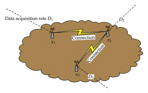
For reliability analysis, the following definitions and lemmas are introduced.

Definition 2.1. Wireless sensor network (2.3) is stochastically reliable in mean-square sense if there exists a bounded positive constant C such that for node data variable x(t, r(t)), there is

(2.5)

Definition 2.2. Wireless sensor network (2.3) is asymptotically reliable almost surely if there exists a bounded positive constant C such that

(2.6)

Lemma 2.3 (see [12].)Given any real matrices Q₁, Q₂, Q₃ with appropriate dimensions such that , the following inequality holds:

(2.7)

Lemma 2.4 (Schur complement). Let X = X^T ∈ ℝ^(n+m)×(n+m) be a symmetric matrix given by , where A ∈ ℝ^n×n, B ∈ ℝ^m×n, C ∈ ℝ^m×m, and C is nonsingular, then X is positive definite if and only if C > 0 and A − B^TC⁻¹B > 0.

3. Reliability Analysis

Considering WSN (2.3) with topology switching, since for each different topology, D(r(t)) may be different, thus the equilibrium for network (2.3) will not necessarily be the same. Assuming that for each regime r(t), the equilibrium is given as u^*(r(t)) with

, where u^*(r(t)) can be different or the same for each different regime r(t), thus there is

(3.1)

In order to shift u^*(r(t)) to the origin, define

(3.2)

(3.3)

Therefore g(z(t, k), k) = [g₁(z₁(t, k), k), g₂(z₂(t, k), k), …, g_N(z_N(t, k), k)] ^T and for each regime k ∈ S, there is g(0, k) = 0. Substituting (3.1)–(3.3) into (2.3), we have

(3.4)

Through this substituting, network (2.3) with switching equilibrium u^*(k) is transferred to network (3.4) with common equilibrium 0. Thus we study stability of network (2.3) around equilibria u^*(k) by investigating stability of network (3.4) around origin. For simplicity, we write z(t, k) as z(k) and matrix c(r(t) = k), G(r(t) = k), D(r(t) = k) as c_k, G_k, D_k.

Let P_k, k ∈ S be a series of symmetric positive definite matrices and construct Lyapunov function as follows:

(3.5)

According to infinitesimal generator [11], there is

(3.6)

The “derivative” of Lyapunov function is given by (3.6), and here Q_3k are a series of symmetric positive definite matrices. For the stability analysis, we will discuss its property from two situations: u^*(k) ≡ u^*(l), which means for each possible topology, the WSN acquires the same quantity of data from environment, and u^*(k) ≠ u^*(l), k, l ∈ S where the WSN acquires different quantity of data because of topology switching.

3.1. Constant Date Acquisition Rate

Consider the date acquisition rate is constant, which means D(k) ≡ D(l) and u^*(k) ≡ u^*(l), for all k, l ∈ S, thus (3.6) has the following form:

(3.7)

In [13], Lasalle theorem of stochastic version was deduced for nonjump case and this theorem can be extended to Markovian jump case as follows.

Theorem 3.1 (Lasalle theorem). Consider Markovian jump system (3.4) with u^*(k) ≡ u^*(l), for all k, l ∈ S, and Lyapunov function V(x(t, k), t, k) satisfies that V(x(t, k), t, k) ∈ C^2,1 (ℝⁿ × ℝ₊ × S; ℝ₊), if there exists 𝒦_∞ function W₁(x(t, k)), W₂(x(t, k)) and nonnegative continuous function W(x(t, k)) such that

(3.8)

then the following equation stands:

(3.9)

Proof. Please refer to the appendix.

By combining Theorem 3.1 and (3.7), we have the following theorem about the stability for network (2.3) with unique equilibrium.

Theorem 3.2. Consider wireless sensor network (2.3) with constant date acquisition rate D, if there exist a series of symmetric positive definite matrices P_k, Q_3k, k ∈ S such that

(3.10)

the network (2.3) is asymptotically reliable almost surely, that is, there is

(3.11)

where J_k is defined as

(3.12)

Proof. Since u^*(k) ≡ u^*(l) = u^*, for all k, l ∈ S, thus (3.6) is translated to

(3.13)

By checking the definition of V(z(k), t, k), ℒV(z(k), t, k) and applying Lemma 2.3 as well as Lemma 2.4, we have immediately:

(3.14)

And it is easily seen that W(z(t, k)) is a classic 𝒦 function of z(t, k). According to the quality of 𝒦 function (seen in [14]), W(z(t, k)) is strictly positive if z(t, k) ≠ 0, thus W(z(t, k)) = 0 implies that z(t, k) = 0, which means sample set {ω : W(z(t, k)) = 0}⊆{ω : z(t, k) = 0} and we have

(3.15)

Combined with (3.14), the following stands:

(3.16)

Immediately we have

(3.17)

3.2. Varying Date Acquisition Rate

In most cases, the distribution of equilibria u^*(k) will differ with different network topology. Obviously this difference will bring effects on the trajectory of node state in network (2.3). For example, network regime is r(t₁) = k at time point t₁ and behavior of state trajectory is determined by the corresponding dynamic , t ≥ t₁ such that the trajectory x(t) is going towards the desired equilibrium u^*(k) with reliability criteria satisfied. After a random time Δt, a sudden event occurs and now the regime is l with new network topology described as , t ≥ t₁ + Δt; thus the trajectory x(t) will going towards a new equilibrium u^*(l) following the new topology. Intuitively, node state x(t) will keep going towards the corresponding equilibrium u^*(j) for each regime j with reliability criteria ensured. Thus it will finally run into a region which is concerned with the distribution of all the equilibria. It is obvious that reliability criteria only guarantee the node trajectory goes towards the equilibrium and cannot explain how close it can be near the equilibrium. For quantitative analysis, we have the following theorem.

Theorem 3.3. Consider stochastic network (2.3) with switching equilibria u^*(k), if there exist a series of symmetric positive-definite matrices P_k, Q_3k and positive scalar ϵ_k such that the following inequality is ensured:

(3.18)

This network is stochastically reliable in mean-square sense, that is, there exists a positive constant C such that

(3.19)

where J_k is defined as

(3.20)

Constant C is determined by u^*(k) with network parameters f(k), G_k, c_k given and P_k, Q_3k, ϵ_k taken.

Proof. According to inequality (3.6), there is

(3.21)

where

(3.22)

Similar to [15], apply generalized Itô formula and result that

(3.23)

Substitute (3.21) into (3.23) and we have

(3.24)

which immediately generates

(3.25)

Let t → ∞ in above inequality, there is

(3.26)

The proof is complete.

Remark 3.4. In above analysis, we give the sufficient conditions for network (2.3) to be reliable in mean-square sense. It can be seen with (3.18) ensured, the trajectory of each regime k is sure to enter an attractive region around the equilibrium u^*(k), and the radius of attractive region is an increasing function of the distance of all equilibria , and this distance reflects the intrinsic characteristic of network which is determined by network topology. In order to decrease the radius, one possible way is to increase the value of α. From (3.25), we know that α determines how fast the trajectory can converge to the attractive region, and α is concerned with node calculation capacity f, network topology G, and network status c. The larger the parameter α is, the faster the convergence speed is, and also the smaller radius is. For these reasons, we request a larger parameter α for convergence speed and convergence precision.

Remark 3.5. Neither control variable nor decision action appears in the model of network (2.3), and the above analysis reflects the natural property of autonomous network. Note that parameter C is a conservative result for the bound of node state, and the radius of attractive region for practical network will be less than C. Consider a network with performance demand that E{|x(t)|²} ≤ γ after calculating we know C ≤ γ; thus we need to do nothing and just let the network work by itself. Otherwise, there may be a need taking control or decision to change either the network topology G_k or the transition rate matrix Π for the satisfaction of performance. This work will be of some help for network topology design and decision making.

4. Numerical Example

Consider the following 2-regime wireless sensor network as shown in Figure 2:

(4.1)

where this network consists of 6 nodes (N = 6), and its topology switches between regime 1 and regime 2 with transition rate matrix as

. Initial node state is x(0) = [10,20, −10, −20, −7,33] ^T and parameters are given as

(4.2)

f₁ = −diag (6 + 1/20, 6 + 2/20, 6 + 3/20, 6 + 4/20, 6 + 5/20, 6 + 6/20)x(t),

(4.3)

f₂ = −diag (1 + 1/10, 1 + 2/10, 1 + 3/10, 1 + 4/10, 1 + 5/10, 1 + 6/10)x(t), and m = 6 for both regimes. For comparison of unique equilibrium case and multiple equilibria case, we adopt the same sample path, that is, Markovian jump is the same throughout numerical experiments as in Figure 3.

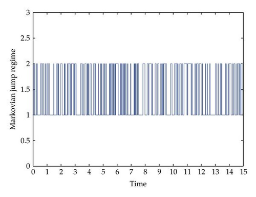
4.1. Constant Date Acquisition Rate

We investigate network (2.3) with unique equilibrium

, i = 1, …, 6, where D₁ = D₂ = [0,0, 0,0, 0,0] ^T. It is easy to see that positive definite matric P₁ = P₂ = Q₃₁ = Q₃₂ = I can satisfy

(4.4)

Thus all the parameters satisfy the reliability criteria in Theorem 3.2, and node state trajectory is shown as follows in Figure 4.

4.2. Varying Date Acquisition Rate

In this subsection, we simulate the case that Markovian jumps change not only the topology structure of network, but also date acquisition rate. And this network has two regimes with two different equilibria:

, i = 1,2, …, 6 with D₁ = 0, D₂ = [5.4861,5.9917,6.4861,6.9972,7.5194,8.0194] ^T. Positive definite matric P₁ = P₂ = Q₃₁ = Q₃₂ = I and scalar ϵ₁ = 0.2, ϵ₂ = 0.5 can satisfy

(4.5)

Thus all the parameters satisfy the reliability criteria in Theorem 3.3, and node sate trajectory is shown in Figure 5

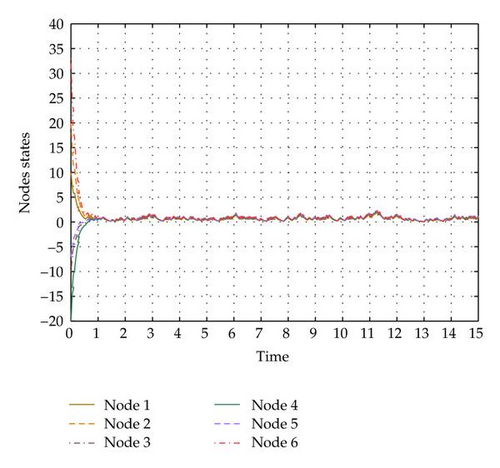
Consider network (2.3) has multiple equilibria , , i = 1, …, 6, thus D₁ = [0,0, 0,0, 0,0] ^T, D₂ = [10.9722,11.9833,12.9722,13,9944,15.0389,16.0389] ^T while other parameters keep unchanged as well as the Markovian jump sample. Noticing that the reliability criteria are the same as the case of , , i = 1,2, …, 6. According to Theorem 3.3, such network is also stable in mean-square sense, and its node state trajectory is shown in Figure 6.

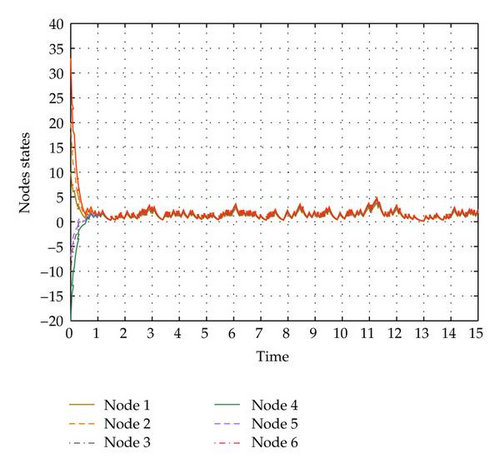
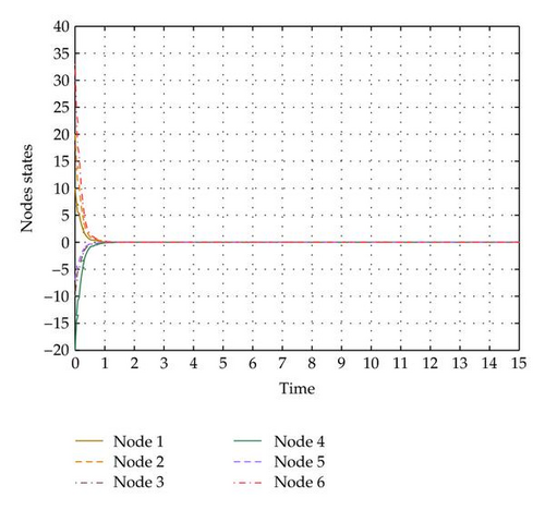
It can be seen from Figures 5 and 6 that with the same parameters P₁, P₂, Q₃₁, Q₃₂, ε₁, ε₂ satisfying the reliability criteria in Theorem 3.2, the node state trajectory can converge to the attractive region with the same convergence speed, which is dependent on parameter f(k), G_k, c_k, N, m, Π with the same P_k, Q_3k, ε_k, that is, this speed is determined by the natural property of network. However, the radius of this region is different: for the former case , , the radius is smaller while for the latter case , , the radius is larger, which means the radius of attractive region is an increasing function of the distance between the equilibria.

5. Conclusion

Reliability problems of stochastically switching wireless sensor network are studied in this paper. This switching, governed by Markovian chain, changes not only network topology, but also the data acquisition rate from outside environment. Our work reveals that reliability is dependent on three elements: network topology, network parameters and Markovian chain. When data acquisition rate keeps unchanged so that all network topologies share a common equilibrium despite of regime jump, network node state can be asymptotically reliable almost surely if the above three elements satisfy sufficient conditions. For varying data acquisition rate case, node state can converge to an attractive region similarly with sufficient conditions ensured, while its radius is concerned with the distribution of all the equilibria. Numerical simulations present an intuitive understanding of these relations and all the reliability criteria in this paper can be feasible for a general network.

Acknowledgments

This work is supported by the National Natural Science Foundation of China under Grant 60904021, the Fundamental Research Funds for the Central Universities under Grant WK2100060004, and National High-Tech Research and Development Program of China 863 Program under Grant 2008AA01A317.

Appendix

Lasalle Theorem in Markovian Jump Systems

Lemma A.1 (Supermartingale inequality [16]). Let ξ_t, t ∈ ℝ₊ be a right-continuous supermartingale, there is for all s₀ < t₀ ∈ ℝ₊, λ > 0, one has

(A.1)

Lemma A.2 (Fatou′s lemma). Let {f_k(x)} be a series of measurable nonnegative functions defined on ℝⁿ, one has

(A.2)

Now we introduce the Lasalle theorem in Markovian jump systems as follows.

Theorem A.3 (Lasalle theorem). Considering Markovian jump system of the form:

(A.3)

where B(t) is a standard Wiener process which is independent of Markov process r(t), suppose there exist a function V(x, t, i) ∈ C^2,1(ℝⁿ × ℝ₊ × S; ℝ₊) and class 𝒦_∞ functions W₁, W₂, such that

(A.4)

(A.5)

where W(·) ∈ C(ℝⁿ; ℝ₊). Then the equilibrium x = 0 is globally stable in probability and there is

(A.6)

Proof. First we will prove the global stability in probability of the Markovian jump system (A.3).

By (A.4) and (A.5), we have ℒV ≤ 0 and V ≥ 0,which means V is a supermartingale on probability space (Ω, ℱ, {ℱ_t} _t≥0, P). For any class 𝒦_∞ function γ(·), with supermartingale inequality applied, there is

(A.7)

According to the quality of 𝒦_∞ function, we have

(A.8)

Connect the above inequality with (A.4) and (A.7)

(A.9)

Thus there is

(A.10)

For any given ζ > 0, choose γ(·) such that

(A.11)

Then we have

(A.12)

and the global stability in probability is proved.

Next we would prove the establishment of (A.6).

We decompose the sample space into three mutually exclusive events:

(1) A₁ = {ω : limsup _t→∞ W(x(t, ω)) = 0},
(2) A₂ = {ω : liminf _t→∞W(x(t, ω)) > 0},
(3) A₃ = {ω : liminf _t→∞W(x(t, ω)) = 0 and limsup _t→∞W(x(t, ω)) > 0}.

and our aim is to prove that P{A₂} = P{A₃} = 0.

Let h = 1,2, … be a positive integer. Define the stopping time as

(A.13)

and it could been easily seen that as h → ∞, τ_h → ∞ (a.s.). According to (A.10) we have

(A.14)

By generalized Itô formula and (A.5)

(A.15)

Here t_h is defined as t_h = t∧τ_h, for all t ≥ 0. Since

, therefore,

(A.16)

Let t → ∞, h → ∞, by applying Fatou’s lemma, there is

(A.17)

Hence

(A.18)

which follows immediately that P{A₂} = 0.

Now we proceed to show that P{A₃} = 0 by contradiction. Suppose P{A₃} > 0, then there exists ϵ > 0 such that

(A.19)

It is easily seen that P{Ω₁∩A₃} ≥ 2ϵ. We now define a sequence of stopping times

(A.20)

By hypothesis (H), for any |x | ≤ h, there exists a constant K_h > 0 such that

(A.21)

From (A.3), we compute

(A.22)

Since W(·) is continuous in ℝⁿ, it must be uniformly continuous in the closed ball B_h = {x ∈ ℝⁿ : |x| ≤ h}. We can therefore choose δ = δ(ϵ) > 0 small enough such that

(A.23)

We furthermore choose T = T(ϵ, δ, h) sufficiently small for

(A.24)

By Chebyshev’s inequality, it can be deduced that

(A.25)

According to operation principle of sets, we have

(A.26)

Thus

(A.27)

According to (A.23), we have

(A.28)

Define probability sample set as

(A.29)

Let 1(·) denote the indicator function of set, and noticed that σ_2k − σ_2k−1 ≥ T, we derive from (A.18) and (A.26) that

(A.30)

which is a contradiction. Thus P{A₃} = 0. Therefore P{A₁} = 1 and the proof is therefore completed.

References

1 Sohraby K., Minoli D., and Znati T., Wireless Sensor Networks: Technology, Protocols, and Applications, 2007, John Wiley and Sons.
10.1002/047011276X
Google Scholar
2 Dargie W. and Poellabauer C., Fundamentals of Wireless Sensor Networks: Theory and Practice, 2010 , John Wiley and Sons.
10.1002/9780470666388
Google Scholar
3 Zhu H., Luo H., Peng H., Li L., and Luo Q., Complex networks-based energy-efficient evolution model for wireless sensor networks, Chaos, Solitons and Fractals. (2009) 41, no. 4, 1828–1835, 2-s2.0-67349223908, https://doi.org/10.1016/j.chaos.2008.07.032.
10.1016/j.chaos.2008.07.032
Web of Science® Google Scholar
4 Chen H., Tse C. K., and Feng J., Impact of topology on performance and energy efficiency in wireless sensor networks for source extraction, IEEE Transactions on Parallel and Distributed Systems. (2009) 20, no. 6, 886–897, 2-s2.0-65949109494, https://doi.org/10.1109/TPDS.2009.14.
10.1109/TPDS.2009.14
Web of Science® Google Scholar
5 Qureshi H. K., Rizvi S., Saleem M., Khayam S. A., Rakocevic V., and Rajarajan M., Poly: a reliable and energy efficient topology control protocol for wireless sensor networks, Computer Communications. (2011) 34, no. 10, 1235–1242, 2-s2.0-79955711119, https://doi.org/10.1016/j.comcom.2010.12.016.
10.1016/j.comcom.2010.12.016
Web of Science® Google Scholar
6 Stroock D. W., An Introduction to Markov Processes, 2005, Springer, Berlin, Germany, 2126069, ZBL1082.35173.
Google Scholar
7 Mariton M., Jump Linear Systems in Automatic Control, 1990, Marcel-Dekker.
Web of Science® Google Scholar
8 Mao X., Yuan C., and Yin G., Approximations of Euler-Maruyama type for stochastic differential equations with Markovian switching, under non-Lipschitz conditions, Journal of Computational and Applied Mathematics. (2007) 205, no. 2, 936–948, https://doi.org/10.1016/j.cam.2006.01.052, 2329667, ZBL1121.65011.
10.1016/j.cam.2006.01.052
Web of Science® Google Scholar
9 Liu Y., Wang Z., and Liu X., Exponential synchronization of complex networks with Markovian jump and mixed delays, Physics Letters A. (2008) 372, no. 22, 3986–3998, https://doi.org/10.1016/j.physleta.2008.02.085, 2418401, ZBL1220.90040.
10.1016/j.physleta.2008.02.085
CAS Web of Science® Google Scholar
10 Liu M., Ho D. W. C., and Niu Y., Stabilization of Markovian jump linear system over networks with random communication delay, Automatica. (2009) 45, no. 2, 416–421, https://doi.org/10.1016/j.automatica.2008.06.023, 2527337, ZBL1158.93412.
10.1016/j.automatica.2008.06.023
Web of Science® Google Scholar
11 Mao X., Stability of stochastic differential equations with Markovian switching, Stochastic Processes and their Applications. (1999) 79, no. 1, 45–67, https://doi.org/10.1016/S0304%2D4149(98)00070%2D2, 1666831, ZBL0962.60043.
10.1016/S0304-4149(98)00070-2
Web of Science® Google Scholar
12 Liao X., Chen G., and Sanchez E. N., LMI-based approach for asymptotically stability analysis of delayed neural networks, IEEE Transactions on Circuits and Systems I. (2002) 49, no. 7, 1033–1039, https://doi.org/10.1109/TCSI.2002.800842, 1916631.
10.1109/TCSI.2002.800842
Web of Science® Google Scholar
13 Mao X., Stochastic versions of the LaSalle theorem, Journal of Differential Equations. (1999) 153, no. 1, 175–195, https://doi.org/10.1006/jdeq.1998.3552, 1682267, ZBL0921.34057.
10.1006/jdeq.1998.3552
Web of Science® Google Scholar
14 Hassan K. K., Nonlinear Systems, 2002, Prentice Hall.
Google Scholar
15 Yuan C. and Mao X., Robust stability and controllability of stochastic differential delay equations with Markovian switching, Automatica. (2004) 40, no. 3, 343–354, https://doi.org/10.1016/j.automatica.2003.10.012, 2145263, ZBL1040.93069.
10.1016/j.automatica.2003.10.012
Web of Science® Google Scholar
16 Øksendal B., Stochastic Differential Equations, 2000, Springer, New York, NY, USA.
Google Scholar

Citing Literature

All articles

Reliability Analysis of Wireless Sensor Networks Using Markovian Model

Abstract

1. Introduction

2. System Model Description