Nonnegativity Preserving Interpolation by C1 Bivariate Rational Spline Surface
Abstract
This paper is concerned with the nonnegativity preserving interpolation of data on rectangular grids. The function is a kind of bivariate rational interpolation spline with parameters, which is C1 in the whole interpolation region. Sufficient conditions are derived on coefficients in the rational spline to ensure that the surfaces are always nonnegative if the original data are nonnegative. The gradients at the data sites are modified if necessary to ensure that the nonnegativity conditions are fulfilled. Some numerical examples are illustrated in the end of this paper.
1. Introduction
Interpolation to the scientific data is of great significance in the area of computer-aided geometric design. Particularly, there is often some property inherent in the data which one wishes to preserve when the interpolant is visualized. One useful shape property is nonnegativity: one may have all data values nonnegative and seek an interpolant that is everywhere nonnegative. In this paper, we are concerned with the nonnegativity preserving bivariate interpolation to data on a rectangular grid.
Several kinds of surfaces are concerned with nonnegativity preserving interpolation on rectangular grid. For example, C1 biquadratic splines on a refined rectangular grid have been considered in paper [1]. In paper [2, 3], Brodlie et al. followed the same approach (but for bicubic interpolation) of maintaining nonnegativity by modifying estimated slopes at data points. In [4], the interpolant is piecewise an average of two blending surfaces. In [5], C1 interpolating surface is constructed piecewise as a convex combination of two bicubic Bézier patches with the same set of boundary Bézier ordinates. Sufficient nonnegativity conditions on the Bézier ordinates are derived to ensure the nonnegativity of a bicubic Bézier patch. The Bézier ordinates are modified locally to fulfill the sufficient nonnegativity conditions.
The surface we consider here is rational spline. Rational spline with parameters has been considered in recent years. Those kinds of interpolation splines have simple and explicit mathematical representation. In paper [6], a bivariate rational interpolation is constructed using both function values and partial derivatives of the function being interpolated as the interpolation data. The convexity control method and point control method have been studied in [7, 8]. In paper [9], a rational cubic function is extended to a rational bicubic partially blended functions (Coons-patches) and the constraints on parameters are derived to visualize the shape of nonnegative surface data. In this paper, we consider the rational spline from different points of view. The sufficient nonnegativity conditions of the bicubic Bézier patch are introduced to consider this problem. We get the sufficient nonnegativity conditions of the rational spline. Gradients at data sites are modified if necessary to ensure that the nonnegativity conditions are fulfilled. It is designed in such a way that no additional points need to be supplied and the sufficient conditions are simple and explicit.
The paper is organized as follows. In Section 2, the bivariate rational spline is introduced. Section 3 deals with the smoothness of the interpolating surface. In Section 4, the sufficient nonnegativity conditions of the rational spline are derived and a local scheme for C1 nonnegativity preserving interpolation is described. We conclude in Section 5 by illustrating the method with some graphical examples.
2. Rational Interpolation Spline
In this section, the univariate rational cubic spline is introduced which was developed by Hussain and Sarfraz [10]. We extend it to a bivariate rational interpolation spline function.
Let Ω : [a, b; c, d] be a planar region, {(xi, yj, fi,j, ∂fi,j/∂x, ∂fi,j/∂y), (i = 1,2, …, n; j = 1,2, …, m)} a given set of data points, where a = x1 < x2 < ···<xn = b and c = y1 < y2 < ···<ym = d are the knot sequences. And let fi,j, ∂fi,j/∂x, ∂fi,j/∂y represent f(xi, yj), ∂f(xi, yj)/∂x, ∂f(xi, yj)/∂y, respectively. ∂f(xi, yj)/∂x and ∂f(xi, yj)/∂y are not always given; they can be estimated by the method in [11].
It is obvious that di,s(x, ys) satisfies di,s(xr, ys) = ∂fr,s/∂y, r = i, i + 1, s = j, j + 1. And the bivariate rational function Si,j(x, y) satisfies the interpolation conditions Si,j(xr, ys) = f(xr, ys), ∂Si,j(xr, ys)/ ∂x = ∂fr,s/∂x, ∂Si,j(xr, yj)/∂y = ∂fr,s/∂y, r = i, i + 1 and s = j, j + 1.
3. The Smoothing Conditions
In this section, the smoothing conditions of the rational spline Si,j(x, y) defined by (2.4) are derived. The rational interpolating function defined by (2.1) is a piecewise Hermite interpolant, and it has continuous first-order derivative when x ∈ [x1, xn]. So the bivariate interpolating function Si,j defined by (2.4) has continuous first-order partial derivatives ∂Si,j(x, y)/∂x and ∂Si,j(x, y)/∂y in the interpolating region [x1, xn; y1, ym] except ∂Si,j(x, y)/∂x at the points (xi, y), i = 1,2, …, n − 1 for every y ∈ [yj, yj+1], j = 1,2, …, m − 1. So it is sufficient for Si,j(x, y) ∈ C1 in the whole interpolating region [x1, xn; y1, ym] if ∂Si,j(xi+, y)/∂x = ∂Si,j (xi−, y)/∂x holds. This leads to the following theorem.
Theorem 3.1. If the knots are equally spaced for variable x; that is, hi = (b − a)/n, a sufficient condition for the interpolating function Si,j(x, y), i = 1,2, …, n − 1; j = 1,2, …, m − 1, to be C1 in the whole interpolating region [x1, xm; y1, yn] is that the parameters μi,j = constant, ωi,j = constant, and αi,j + βi−1,j = 2 for each j ∈ [1,2, …, m − 1] and all i = 1,2, …, n − 1.
Proof. From the analysis above, without loss of generality, for any pair (i, j), 1 ≤ i ≤ n − 1, 1 ≤ j ≤ m − 1, and y ∈ [yj, yj+1], it is sufficient to prove
If (3.1) holds, it needs (3.5) = (3.7); it can be seen that μi,j = μi−1,j, ωi,j = ωi−1,j, αi,j + βi−1,j = 2, and hi = hi−1.
This completes the proof.
The interpolating scheme above begins in x-direction first. If the interpolation begins with y-direction first, we would get a restriction on the data in the y-direction.
4. Construction of Nonnegativity Preserving Interpolating Surface
In this section we first introduce the following theorem in paper [5], which is the basis of our discussion below.
Theorem 4.1. Let , where {b0,0, b3,0, b0,3, b3,3} = {αι, βι, γι, ι}, with ι > 0 and α ≥ β ≥ γ ≥ 1. Let λ = γ if ι and γι are values at the diagonal vertices; otherwise λ = β. If b1,0, b2,0, b1,3, b2,3, b0,1, b0,2, b3,1, b3,2, b1,1, b2,1, b1,2, b2,2 ≥ −l/3a, where a is the smallest solution in (1,5] of
It can be seen that is positive for αi,j > 0 and βi,j > 0. The function ti,j is a bicubic Bézier patch. It is nonnegative if the Bézier ordinates of it satisfy the conditions in Theorem 4.1.
Bézier ordinates of ti,j need not to satisfy the nonnegative conditions. To ensure this, we shall impose upon these Bézier ordinates the conditions bp,q ≥ −ι/3a (p, q = 0,1, 2,3) according to Theorem 4.1, where ι = min {fi,j, fi,j+1, fi+1,j, fi+1,j+1} and a is determined by (4.1). This can be achieved by modifying if necessary the gradients at vertices Vi,j = (xi, yj). The modification of derivatives ∂fi,j/∂x and ∂fi,j/∂y at a vertex is performed by scaling each of them with a positive factor α< 1. The scaling factor α is obtained by taking into account all the rectangular patches sharing that vertex. For the four rectangles which share vertex Vi,j, denote vertex Vi,j as O and its adjacent vertices as A, B, C, D, E, F, G, H, respectively (see Figure 1).
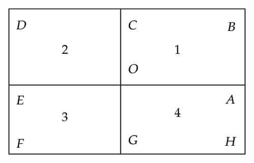
Consider rectangle 1 and the lower bound −ι1/3a1 where ι1 = min {S(O), S(A), S(B), S(C)} and a1 is obtained by solving (4.1) in Theorem 4.1. Scalar is defined as follows. If μi,jfi,j + lj(∂fi,j/∂y)≥−ι1/3a1, then . Otherwise, is defined by the equation . Similarly for the scalar , if αi,jfi,j + hi(∂fi,j/∂x)≥−ι1/3a1, then ; otherwise is given by the equation . For the scalar , if μi,jαi,jfi,j + μi,jhi(∂fi,j/∂x) + lj(∂fi,j/∂y)≥−ι1/3a1, then ; otherwise is determined by the equation . Then define . By using the same argument above, we get α21 and α22, α31 and α32, α41 and α42 for rectangles 2, 3, 4, respectively. In order for all the Bézier ordinates adjacent to O to fulfill the positivity preserving conditions stated in Theorem 4.1, set αO1 = min {α11, α21, α31, α41}, αO2 = min {α12, α22, α32, α42}.
If αO1 < 1 (or αO2 < 1), the x (or y) partial derivatives at O are redefined as αO1(∂fO/∂x) and αO2(∂fO/∂y). Then the Bézier ordinates adjacent to O in each rectangle are redetermined. The above process is repeated at all the nodes Vi,j.
For the boundary node O, which belongs to one or two rectangles of the rectangular grid, αO is defined in a similar way. The only difference is that we consider only one or two rectangles instead of four.
Now all the Bézier ordinates are determined, so ti,j is nonnegative. Thus we can get the C1 rational interpolant S, which is nonnegative.
5. Numerical Examples
We shall illustrate our discussion with the following examples.
Example 5.1. In the first example the data are given as follows:
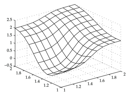
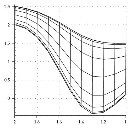
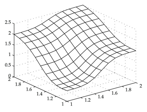
Figure 2 shows the rational interpolation surface, which loses the nonnegativity in its display. Figure 3 is a different view of Figure 2 after making a rotation. It confirms that the surface is not preserving nonnegativity feature. Figures 4 and 5 show the surface after modifying by the scheme of this paper, which are indeed nonnegative. In fact, they are changed as follows:
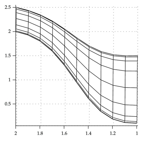
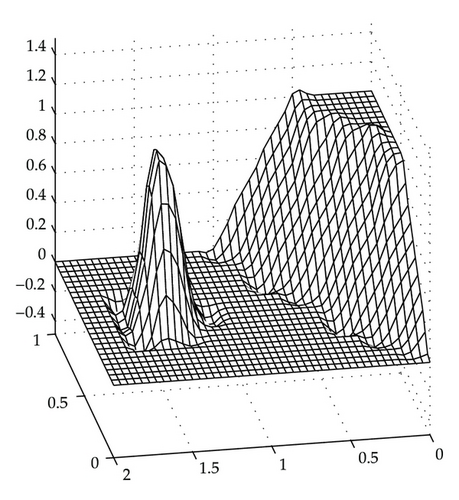
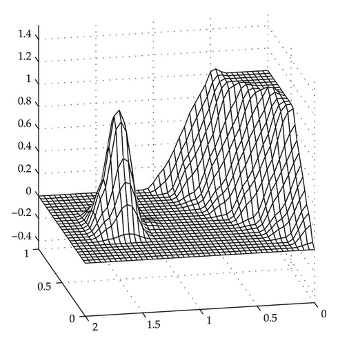
Example 5.2. In the second example, data points are generated from function g(x, y) [12]:
Figure 6 shows the unconstrained interpolating surface, which loses the nonnegativity in its display. Output from the nonnegativity preserving scheme of this paper is shown in Figure 7. It clearly shows that the surface remains nonnegative everywhere and visually pleasant.
6. Conclusion
In this paper, we construct a nonnegativity preserving interpolant of data on rectangular grids by using the rational spline. The sufficient nonnegativity conditions are derived, which are simple and explicit. And the experimental results illustrate the feasibility and validity of our method.
Acknowledgment
The authors acknowledge the financial support of the Liaoning Educational Committee (L2010221).


