Robust Adaptive Switching Control for Markovian Jump Nonlinear Systems via Backstepping Technique
Abstract
This paper investigates robust adaptive switching controller design for Markovian jump nonlinear systems with unmodeled dynamics and Wiener noise. The concerned system is of strict-feedback form, and the statistics information of noise is unknown due to practical limitation. With the ordinary input-to-state stability (ISS) extended to jump case, stochastic Lyapunov stability criterion is proposed. By using backstepping technique and stochastic small-gain theorem, a switching controller is designed such that stochastic stability is ensured. Also system states will converge to an attractive region whose radius can be made as small as possible with appropriate control parameters chosen. A simulation example illustrates the validity of this method.
1. Introduction
The establishment of modern control theory is contributed by state space analysis method which was introduced by Kalman in 1960s. This method, describing the changes of internal system states accurately through setting up the relationship of internal system variables and external system variables in time domain, has become the most important tool in system analysis. However, there remain many complex systems whose states are driven by not only continuous time but also a series of discrete events. Such systems are named hybrid systems whose dynamics vary with abrupt event occurring. Further, if the occurring of these events is governed by a Markov chain, the hybrid systems are called Markovian jump systems. As one branch of modern control theory, the study of Markovian jump systems has aroused lots of attention with fruitful results achieved for linear case, for example, stability analysis [1, 2], filtering [3, 4] and controller design [5, 6], and so forth. But studies are far from complete because researchers are facing big challenges while dealing with the nonlinear case of such complicated systems.
The difficulties may result from several aspects for the study of Markovian jump nonlinear systems (MJNSs). First of all, controller design largely relies on the specific model of systems, and it is almost impossible to find out one general controller which can stabilize all nonlinear systems despite of their forms. Secondly Markovian jump systems are applied to model systems suffering sudden changes of working environment or system dynamics. For this reason, practical jump systems are usually accompanied by uncertainties, and it is hard to describe these uncertainties with precise mathematical model. Finally, noise disturbance is an important factor to be considered. More often that not, the statistics information of noise is unknown when taking into account the complexity of working environment. Among the achievements of MJNSs, the format of nonlinear systems should be firstly taken into account. As one specific model, the nonlinear system of strict-feedback form is well studied due to its powerful modelling ability of many practical systems, for example, power converter [7], satellite attitude [8], and electrohydraulic servosystem [9]. However, such models should be modified since stochastic structure variations exist in these practical systems, and this specific nonlinear system has been extended to jump case. For Markovian jump nonlinear systems of strict-feedback form, [10, 11] investigated stabilization and tracking problems for such MJNSs, respectively. And [12] studied the robust controller design for such systems with unmodeled dynamics. However, for the MJNSs suffering aforementioned factors in this paragraph, research work has not been performed yet.
Motivated by this, this paper focuses on robust adaptive controller design for a class of MJNSs with uncertainties and Wiener noise. Compared with the existing result in [12], several practical limitations are considered which include the following: the uncertainties are with unmodeled dynamics, and the upper bound of dynamics is not necessarily known. Meanwhile the statistics information of Wiener noise is unknown. Also the adaptive parameter is introduced to the controller design whose advantage has been described in [13]. The control strategy consists of several steps: firstly, by applying generalized formula, the stochastic differential equation for MJNS is deduced and the concept of JISpS (jump input-to-state practical stability) is defined. Then with backstepping technology and small-gain theorem, robust adaptive switching controller is designed for such strict-feedback system. Also the upper bound of the uncertainties can be estimated. Finally according to the stochastic Lyapunov criteria, it is shown that all signals of the closed-loop system are globally uniformly bounded in probability. Moreover, system states can converge to an attractive region whose radius can be made as small as possible with appropriate control parameters chosen.
The rest of this paper is organized as follows. Section 2 begins with some mathematical notions including differential equation for MJNS, and we introduce the notion of JISpS and stochastic Lyapunov stability criterion. Section 3 presents the problem description, and a robust adaptive switching controller is given based on backstepping technique and stochastic small-gain theorem. In Section 4, stochastic Lyapunov criteria are applied for the stability analysis. Numerical examples are given to illustrate the validity of this design in Section 5. Finally, a brief conclusion is drawn in Section 6.
2. Mathematical Notions
2.1. Stochastic Differential Equation of MJNS
Throughout the paper, unless otherwise specified, we denote by a complete probability space with a filtration satisfying the usual conditions (i.e., it is right continuous and ℱ0 contains all p-null sets). Let |x| stand for the usual Euclidean norm for a vector x, and let ∥xt∥ stand for the supremum of vector x over time period [t0, t], that is, . The superscript T will denote transpose and we refer to Tr (·) as the trace for matrix. In addition, we use L2(P) to denote the space of Lebesgue square integrable vector.
Remark 2.1. Equation (2.7) is the differential equation of MJNS (2.1). It is given by [12], and the similar result is also achieved in [15]. Compared with the differential equation of general nonjump systems, two parts come forth as differences: transition rates πkj and martingale process M(t), which are both caused by the Markov chain r(t). And we will show in the following section that the martingale process also has effects on the controller design.
2.2. JISpS and Stochastic Small-Gain Theorem
Definition 2.2. MJNS (2.1) is JISpS in probability if for any given ϵ > 0, there exist 𝒦ℒ function β(·, ·), 𝒦∞ function γ(·), and a constant dc ≥ 0 such that
Remark 2.3. The definition of ISpS (input-to-state practically stable) in probability for nonjump stochastic system is put forward by Wu et al. [16], and the difference between JISpS in probability and ISpS in probability lies in the expressions of system state x(t, k) and control signal ut(k). For nonjump system, system state and control signal contain only continuous time t with k ≡ 1. While jump systems concern with both continuous time t and discrete regime k. For different regime k, control signal ut(k) will differ with different sample taken even at the same time t, and that is the reason why the controller is called a switching one. Based on this, the corresponding stability is called Jump ISpS, and it is an extension of ISpS. Let k ≡ 1, and the definition of JISpS will degenerate to ISpS.
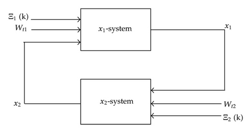
Lemma 2.4 (stochastic small-gain theorem). Suppose that both the x1-system and x2-system are JISpS in probability with (Ξ1(k), x2(t, k)) as input and x1(t, k) as state and (Ξ2(k), x1(t, k)) as input and x2(t, k) as state, respectively; that is, for any given ϵ1, ϵ2 > 0,
If there exist nonnegative parameters ρ1, ρ2, s0 such that nonlinear gain functions γ1, γ2 satisfy
Remark 2.5. The previously mentioned stochastic small-gain theorem for jump systems is an extension of nonjump case. This extension can be achieved without any mathematical difficulties, and the proof process is the same as in [16]. The reason is that in Lemma 3.1 we only take into account the interconnection relationship between synthetical system and its subsystems, despite the fact that subsystems are of jump or nonjumpform. If both subsystems are nonjump and ISpS in probability, respectively, the synthetical system is ISpS in probability. By contraries, if both subsystems are jump and JISpS in probability, respectively, the synthetical system is JISpS in probability correspondingly.
3. Problem Description and Controller Design
3.1. Problem Description
- (A1)
The ξ subsystem with input y is JISpS in probability; namely, for any given ϵ > 0, there exist 𝒦ℒ function β(·, ·), 𝒦∞ function γ(·), and a constant dc ≥ 0 such that
() - (A2)
For each i = 1,2, …, n, k ∈ S, there exists an unknown bounded positive constant such that
()where , are known nonnegative smooth functions for any given k ∈ S. Notice that is not unique since any satisfies inequality (3.3). To avoid confusion, we define the smallest nonnegative constant such that inequality (3.3) is satisfied.
For the design of switching controller, we introduce the following lemmas.
Lemma 3.1 (Young’s inequality [12]). For any two vectors x, y ∈ ℝn, the following inequality holds
Lemma 3.2 (martingale representation [17]). Let B(t) = [B1(t), B2(t), …, BN(t)] be N-dimensional standard Wiener noise. Supposing M(t) is an -martingale (with respect to P) and that M(t) ∈ L2(P) for all t ≥ 0, then there exists a stochastic process Ψ(t) ∈ L2(P), such that
3.2. Controller Design
4. Stochastic Stability Analysis
Theorem 4.1. Considering the MJNS (3.1) with Assumptions (A2) standing, the X-subsystem is JISpS in probability with the adaptive laws (3.14) and switching control law (3.16) adopted; meanwhile all solutions of closed-loop X-subsystem are ultimately bounded.
Proof. Considering the MJNS (3.1) with Lyapunov function (3.11), the following equations hold according to [10]:
For each integer h ≥ 1, define a stopping time as
The proof is completed.
Theorem 4.2. Considering the MJNS (3.1) with Assumptions (A1), (A2) holding, the interconnected Markovian jump system is JISpS in probability with adaptive laws (3.14) and switching control law (3.16) adopted; meanwhile all solutions of closed-loop system are ultimately bounded. Furthermore, the system output could be regulated to an arbitrarily small neighborhood of the equilibrium point in probability within finite time.
Proof. From Assumption (A1), the ξ subsystem is JISpS in probability. And it has been shown in Theorem 4.1 that the X subsystem is JISpS in probability. Similar to the proof in [12], we have that the entire MJNS (3.1) is JISpS in probability; that is, for any given ϵ > 0, there exists T > 0 and δ > 0 such that if t > T, the output of jump system y satisfies
5. Simulation
Case 1. The system regime is k = 1:
Case 2. The system regime is k = 2:
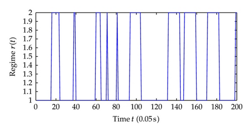
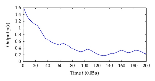
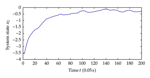
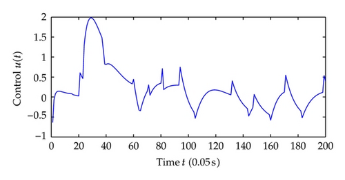
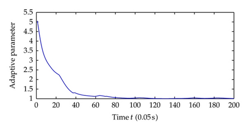
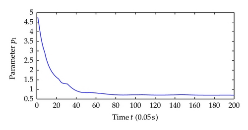
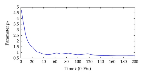
Now we choose different control parameters as c1 = c2 = 2, σ1 = σ2 = 5 and repeat the simulation. The simulation results are as follows. Figure 9 shows the regime transition of the jump system, Figure 10 shows the system output y which is defined as the system state x1 and, Figure 11 shows system state x2, and Figure 12 shows the corresponding switching controller u; the trajectory of adaptive parameter θ is shown in Figures 13 and 14; Figure 15 shows the trajectory of parameter p1, p2, respectively.
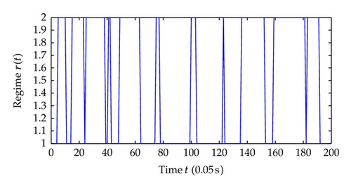
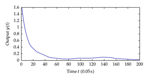
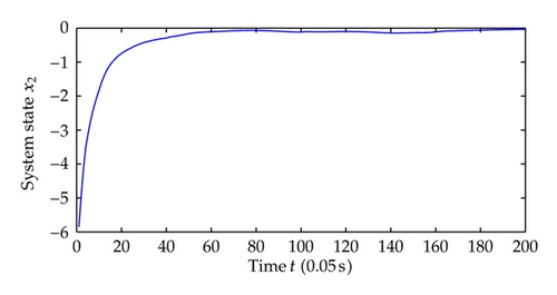
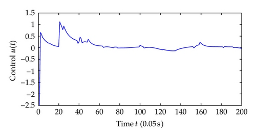
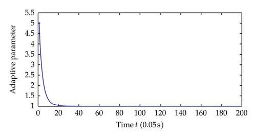
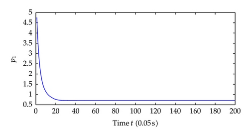
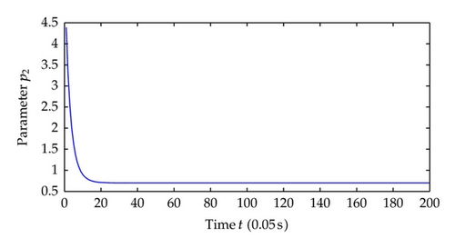
Comparing the results from two simulations, all the signals of closed-loop system are globally uniformly ultimately bounded, and the system output can be regulated to a neighborhood near the equilibrium point despite different jump samples. As could be seen from the figures, larger values of c1, c2, σ1, σ2 help to increase the convergence speed of system states. This reason is that the increase of these parameters increases the value of α, which determines the system states convergence speed. Also adaptive parameters θ and p1, p2 approach convergence faster with the increasing of aforementioned parameters.
Remark 5.1. Much research work has been performed towards the study of nonlinear system by using small-gain theorem [16, 19]. In contrast to their contributions, this paper considers a more general form than nonjump systems. The controller u(k) varies with different regime r(t) = k taken, and it differs in two aspects (see (3.16)): the coupling of regimes πkjαi−1(j) and , which are both caused by the Markovian jumps. The switching controller will degenerate to an ordinary one if r(t) ≡ 1. This controller design method can also be applied for the nonjump nonlinear system.
6. Conclusion
In this paper, the robust adaptive switching controller design for a class of Markovian jump nonlinear system is studied. Such MJNSs, suffering from unmodeled dynamics and noise of unknown covariance, are of the strict feedback form. With the extension of input-to-state stability (ISpS) to jump case as well as the small-gain theorem, stochastic Lyapunov stability criterion is put forward. By using backstepping technique, a switching controller is designed which ensures the jump nonlinear system to be jump ISpS in probability. Moreover the upper bound of uncertainties can be estimated, and system output will converge to an attractive region around the equilibrium point, whose radius can be made as small as possible with appropriate control parameters chosen. Numerical examples are given to show the effectiveness of the proposed design.
Acknowledgment
This work is supported by the National Natural Science Foundation of China under Grants 60904021 and the Fundamental Research Funds for the Central Universities under Grants WK2100060004.


