Energy-Driven Image Interpolation Using Gaussian Process Regression
Abstract
Image interpolation, as a method of obtaining a high-resolution image from the corresponding low-resolution image, is a classical problem in image processing. In this paper, we propose a novel energy-driven interpolation algorithm employing Gaussian process regression. In our algorithm, each interpolated pixel is predicted by a combination of two information sources: first is a statistical model adopted to mine underlying information, and second is an energy computation technique used to acquire information on pixel properties. We further demonstrate that our algorithm can not only achieve image interpolation, but also reduce noise in the original image. Our experiments show that the proposed algorithm can achieve encouraging performance in terms of image visualization and quantitative measures.
1. Introduction
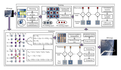
Image interpolation is a very important aspect of image processing and involves the use of a known pixel set to produce an unknown pixel set, resulting in an image of higher resolution [1, 2]. This technique is widely used in remote sensing, aerospace, infrared imaging, low-light level night imagery, and other fields [3–5]. However, maintaining image quality during image interpolation is still a difficult issue [6]. To address this, many image interpolation methods have been proposed. For example, traditional bilinear interpolation computes the unknown pixel value using the location information between the adjacent pixels. This technique does not consider the contents of the image, so edge blurring will occur in the interpolated image [7, 8]. In order to capture image details more clearly, an artifact-free image upscaling method called ICBI [9] has recently been proposed, which uses iterative curvature-based interpolation to obtain a high image quality, but does not take into account underlying local information between image patches. Local image information can be mined according to its structural redundancy characteristic, as proposed by Glasner et al. [10]. This characteristic can lay the foundations for the training and predicting of a statistical model [11, 12]. A statistical model known as Gaussian process regression (GPR) was first applied in the reconstruction of high-resolution images in 2011 and has been shown to be capable of generating an image with sharp edges by extracting the necessary information from a low-resolution image [13]. However, it should be noted that this method only uses the local structural information for each pixel’s neighborhood, so it can still generate unexpected details. To develop the above techniques, we propose here a novel energy-driven interpolation algorithm employing Gaussian process regression (EGPR) (Figure 1). This algorithm not only emphasizes the influence of adjacent pixel properties on interpolated values, but also brings into full play the role of the statistical model.

Our contribution is twofold. Firstly, we propose a framework for both magnification and deblurring in order to fulfill the interpolation task for low-resolution images with low noise. Secondly, we demonstrate an energy-driven approach based on the properties of adjacent pixels within this framework. In addition, we define the processing unit and its properties for better implementation of the EGPR algorithm.
The rest of the paper is structured as follows. Section 2 discusses GPR. Section 3 illustrates the proposed EGPR algorithm. Section 4 presents experimental work carried out to demonstrate the effectiveness of our algorithm. Section 5 concludes the paper.
2. Gaussian Process Regression
3. The Proposed Algorithm
3.1. Training
The following definitions are used in the EGPR algorithm.
Definition 3.1. A given image L is divided into many regions of equal size, and each region is defined as a processing unit (PU). Each PU is also divided into 3 × 3 overlapping image patches (the total number is M). The center of each patch is defined as an output vector YTR of PU, where , while the nearest eight values are defined as an input vector XTR of PU, where
Definition 3.2. Given a total of N pixels in each PU, the pixels are sorted and denoted as I1, I2 … IN. Imax ave, Imin ave, and Iave are defined using the following formulae:
To facilitate the operation of the PU, it is necessary to introduce some properties in advance.
Property 1. Given a number N in each PU, if Imax ave = 0, then pixel value Ii = 0, where i ≤ N.
Property 2. Given xij, if xij = a, then its corresponding output vector value is yij = a, where yij ∈ YTR, i ∈ M, j = 1.
Before applying GPR, we can obtain the particular relationship between the input and output vectors of PU according to Properties 1 and 2. Pixels with this relationship need not be included in the following GPR training, so the predicted values can be directly obtained, saving time and speeding up the EGPR algorithm.
Training plays an important role in the EGPR algorithm, and we adopt a different approach from that used in [13]. Our algorithm contains two processes: training domain establishment and GPR model foundation. In the first stage, we search possible training domains along the four directions of each specific PU. Next, we compute the structural similarity between directions to determine the definite training domain. Inspired by the concept of image SSIM, we define the PU structural similarity as follows.
Definition 3.3 (PU structural similarity). Given two processing units P and Q, their structural similarity is defined as
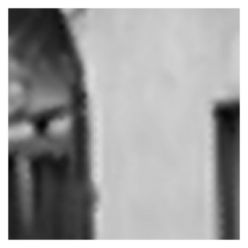
When aiming to achieve high-quality images, the conjugate gradients method is chosen to obtain the model hyperparameters, including mean, variance, and log marginal likelihood. Notice that different iteration numbers in the conjugate gradients method may lead to different prediction accuracies. Figure 3 shows the interpolation images obtained after 50 iterations and 100 iterations, where it can be seen that the latter is better than the former.

3.2. Prediction
Suppose that the low-resolution image Lij is of size m × n and that it is changed to the corresponding interpolated image of size ((m × 2scale) − (2scale − 1)) × ((n × 2scale) − (2scale − 1)), where “scale” denotes the magnification factor. Then we use the nearest interpolation algorithm for the missing pixels in order to obtain the image of size (m × 2scale) × (n × 2scale).
During the prediction of high-resolution image pixels, two rules should be obeyed. Firstly, the PU divided by the initial high-resolution image should correspond to that divided by the low-resolution image. Secondly, the gradient algorithm should satisfy the common positive definite matrix. If not, it will lead to a zero prediction, and the prediction value will need modifying. The modification method can be utilized to maintain the original interpolated pixel value. Finally, we combine all the processing units together in a smooth manner to obtain the high-resolution images without noise.
4. Experimental Results and Discussion
In this section, we compare the experimental results obtained using the proposed algorithm with those obtained using the bilinear algorithm, GPR algorithm [13], and ICBI algorithm [9]. Each algorithm was run in MATLAB. In order to evaluate algorithm performance, we first downsampled original high-quality images to acquire low-resolution images. Then we enlarged these low-resolution images by utilizing the different interpolation algorithms and compared the enlarged images with the original high-quality images. In all experiments, we set the PU size to 30 × 30, but this may be increased according to the magnification factor. At the same time, we used zero mean and square exponential functions as the respective mean and covariance functions in the EGPR. The covariance function required two hyperparameters: a characteristic length scale, the default value of which was 0.21, and the standard deviation of the signal, the default value of which was 0.08. In addition, to achieve color image interpolation, we trained and predicted the GPR model separately for each of the R, G, and B channels.
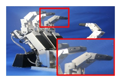
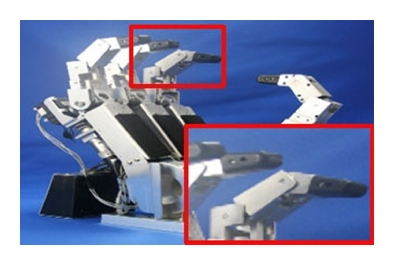
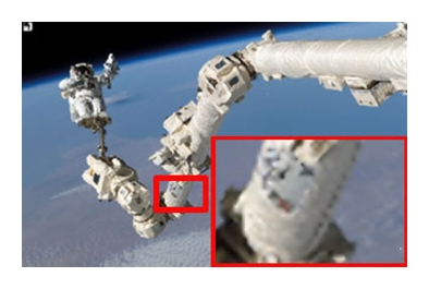
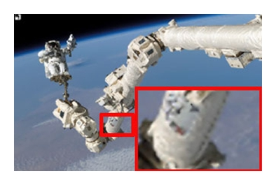
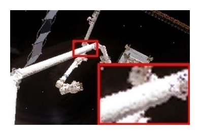
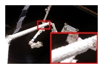
Figure 4 shows the interpolation results from the four algorithms when “scale” was set as 1. Figures 4(a)–4(d) are comparisons of image 1, and Figures 4(e)–4(h) are comparisons of image 2. In the enlarged red-bordered region, it can be seen that the bilinear method introduces jaggy effects, the GPR method reduces these jaggy effects, and the ICBI method achieves a clear edge but is still a little blurry. By employing the energy computation based on properties of adjacent pixels, our new method generates a clearer image without noise.

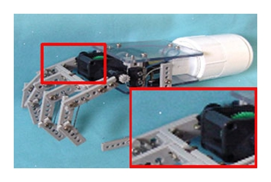


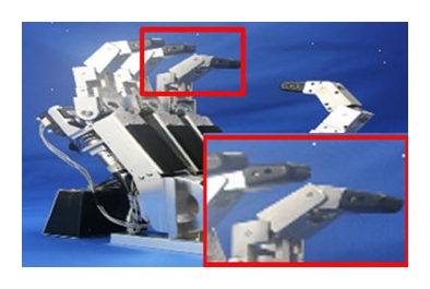
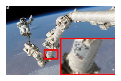
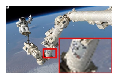
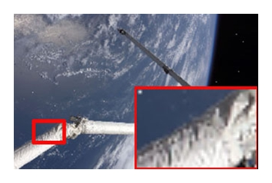
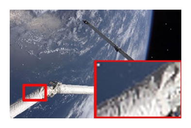
Similarly, Figures 5 and 6 demonstrate the interpolation results with scales of 2 and 3, respectively. From these figures, it can be seen that our method achieved the clearest and smoothest enlarged image of the four methods tested, for example, along edges on the root hand in Figure 6(h). Moreover, the advantages of our proposed algorithm become more enhanced at greater enlargement factors.
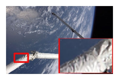
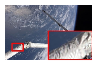
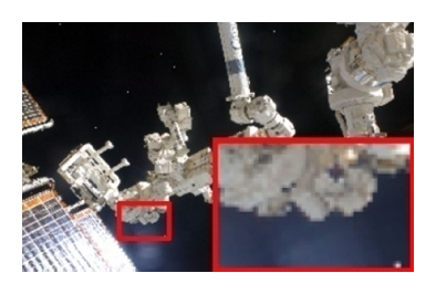


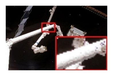

To further validate our algorithm, we also provide objective measurements. Peak signal-to-noise ratio (PSNR) and root mean square (RMS) error are traditional quantitative measures of accuracy, and by comparing their values for the above images, we can conclude that the proposed EGPR algorithm yields interpolated pixel values that are much closer to their original high-quality values than those obtained with the bilinear algorithm, GPR algorithm, and ICBI algorithm. Tables 1 and 2 summarize the PSNR and RMS values for each algorithm at different magnification factors and for each image. It can be observed that the PSNR values for images obtained using the EGPR algorithm are the highest, and those using the bilinear algorithm are the lowest. Further, RMS values for images obtained using the EGPR algorithm are the lowest, and those using the bilinear algorithm are the highest. Overall, it can be clearly demonstrated that our new method outperforms the other three algorithms.
| Image | Scale | Bilinear | GPR | ICBI | EGPR |
|---|---|---|---|---|---|
| Image 1 | 1 | 32.9940 | 33.2792 | 33.3456 | 33.3986 |
| Image 2 | 1 | 30.6314 | 30.7861 | 31.3684 | 31.4594 |
| Image 3 | 2 | 29.5738 | 29.4194 | 29.7173 | 29.7213 |
| Image 4 | 2 | 27.7717 | 27.4767 | 27.8485 | 27.8625 |
| Image 5 | 3 | 23.4038 | 24.4366 | 24.7153 | 24.7171 |
| Image 6 | 3 | 24.3122 | 25.1477 | 25.6880 | 25.6909 |
| Image | Scale | Bilinear | GPR | ICBI | EGPR |
|---|---|---|---|---|---|
| Image 1 | 1 | 16.4437 | 15.8419 | 15.7032 | 15.6004 |
| Image 2 | 1 | 21.1046 | 20.3410 | 19.1890 | 18.9614 |
| Image 3 | 2 | 24.9225 | 24.8861 | 24.4329 | 24.4191 |
| Image 4 | 2 | 31.0516 | 32.1427 | 30.6882 | 30.6118 |
| Image 5 | 3 | 50.8161 | 44.8762 | 43.3017 | 43.2633 |
| Image 6 | 3 | 45.9833 | 41.5720 | 39.0571 | 39.0412 |
MSSIM [25] is an image quality assessment index which assesses the image visibility quality from an image formation point of view under the assumption of the correlation between human visual perception and image structural information. We compared the MSSIM obtained using the EGPR algorithm at different scale values with the corresponding values obtained using the bilinear, GPR, and ICBI algorithms, as shown in Table 3. It is noted that our new algorithm achieves a greater MSSIM than the other three algorithms, and the results show that the images obtained using our algorithm are closer to the original high-resolution images in terms of image structure similarity.
| Image | Scale | Bilinear | GPR | ICBI | EGPR |
|---|---|---|---|---|---|
| Image 1 | 1 | 0.936 | 0.937 | 0.938 | 0.940 |
| Image 2 | 1 | 0.946 | 0.947 | 0.953 | 0.955 |
| Image 3 | 2 | 0.905 | 0.906 | 0.909 | 0.910 |
| Image 4 | 2 | 0.812 | 0.808 | 0.815 | 0.816 |
| Image 5 | 3 | 0.818 | 0.837 | 0.850 | 0.851 |
| Image 6 | 3 | 0.857 | 0.865 | 0.878 | 0.879 |
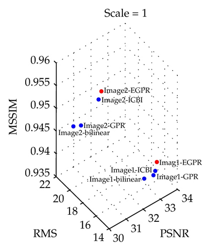
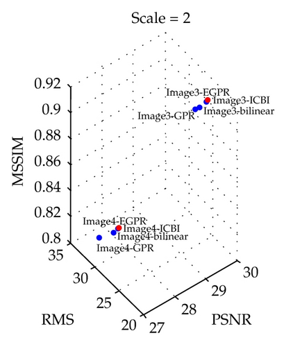
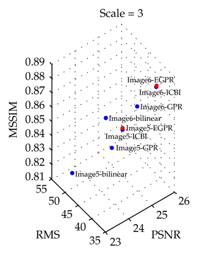
In addition, Figure 7 clearly demonstrates the quantitative assessment results for each image at different magnification levels. In this figure, the blue dots represent the quality scores of the images obtained using the comparison algorithms, and the red dots represent those obtained using our algorithm. Our interpolation algorithm is notably superior to the other algorithms, according to all three objective measurements. The proposed algorithm therefore yielded encouraging performance in terms of image visualization and quantitative quality assessment, making it a competitive image interpolation algorithm.
5. Conclusions
In this paper, we have presented a novel EGPR method for image interpolation. The main feature of this new algorithm is its ability to obtain relatively high prediction accuracy of the unknown pixels by fully utilizing underlying image patch information. The implementation process involves two steps: training and prediction. The former creates a GPR model using only single-image data as the training set, and the latter combines energy computation with the acquired model to produce a high-resolution image. Experiments have shown that our algorithm can yield encouraging performance not only in terms of image visualization but also in terms of PSNR, RMS, and MSSIM quality measures. However, better image interpolation comes at the expense of greater algorithm complexity. Methods of improving the algorithm efficiency need further investigation. In future, we can improve this algorithm to address the problem of the interpolation of image sequences. Images in the same sequence are also subject to the recurrence phenomenon, whereby images contain spatial-temporal correlation [26]. We believe that this problem can be addressed using the improved EGPR algorithm by finding an appropriate energy-driven computation and training mode.
Acknowledgments
This work was supported by the National Basic Research Program of China (973 Program) 2012CB821200 (2012CB821206), the National Natural Science Foundation of China (no. 91024001, no. 61070142), and the Beijing Natural Science Foundation (no. 4111002).


