Model Reference Control for an Economic Growth Cycle Model
Abstract
A useful method in intelligent engineering, called model reference control (MRC), is applied in an economic control problem. The authors review the main framework of MRC and Goodwin growth cycle (GGC) model between two countries and drive the employment rate to be approximate stable in a high level by controlling the workers′ share in the national income automatically. It is very helpful to constitute economic policies for a country or an economic union.
1. Introduction
The control problems in economy are very important for the countries or economic unions. For more than 50 years, methods which were originally created by control engineers and later fully developed by applied mathematicians have been applied to extend the theory of economic policy [1–7]. Control theory can be regarded as a collection of methods to be used by economists, just like statistics and other theories of applied mathematics. There are many economic applications of classical control theories, such as closed-loop system control [5–7], optimal control [2, 3, 8–10], stochastic control [11–14], decentralized control [15, 16], and robust control [17–19]. However, in recent years, classic economic control has become more difficult to implement, as economic behaviors become more and more complex. It is because that these classic control theories are not fit for controlling some complex economic systems. Hence, economists, engineers, and mathematicians have been exploring the possibility that advanced control techniques in engineering would be used in economics as well in these years.
Model reference control (MRC) is a famous intelligent engineering method which has a great use in controlling nonlinear complex systems [20–23]. Also, MRC is widely used in engineering problem with the aid of neural network technique. For example, see [24, 25] for the control of robots, for the control of mechanical oscillators [26], and for flight vehicles [27–29]. In economic application, Etsuo Yamamura and his coauthors published a series of papers on MRC in both theoretical and practical fields in 1980s [30–40]. However, for the limitations of computational methods and computer hardware conditions, they have given many novel ideas and results based on some simple data sets or equations. In recent years, with the development of neural network technology and the improvement of computer performance, the application of MRC has become very simple and efficient; see [41, 42].
The aim of this paper is to expand the MRC to the field of economic control with the aid of neural network technique. The numerical results will show that MRC is an excellent tool for controlling some complex economic systems, such as Goodwin growth cycle (GGC) model between two countries, and, of course, this may be also valuable in constituting economic policies for a country or an economic union as Holt′s work [43] has done. This fully shows the efficiency and practicality of MRC with neural network structure in economic application.
The rest of this paper is organized as follows. In Section 2, we will introduce the theoretic framework of MRC; in Section 3, we will introduce the GGC model between two countries; in Section 4, we will construct a reference model by driving the expected inflation rate to be zero and show an application of MRC to the GGC model; in Section 5, we will conclude our work.
2. Model Reference Control
In this section, we will introduce the theoretic framework of MRC in detail.
2.1. System Identification
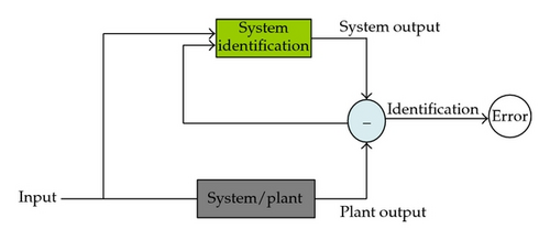
Model reference control includes two parts, system identification and controller generation. The function of system identification is to construct an algorithm for building a model from observed data automatically.
The observed data should be classified as input data and output data which are measured at discrete instants of time t. The observed data set is the training set for system identification process, and we are interested in building the identified model for the purpose of prediction and control [44]. Especially, the identified model may generate accurate prediction values and make a direct connection with the controller.
2.2. Controller Generation
In the following, we will introduce the next process, controller generation part. Here, our main work is to design a controller to drive the plant output to follow the tendency described by the reference model.
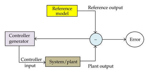
Note that the yellow box represents the reference model with the tendency which we desire for; the pink box represents the controller generator which is used to drive the plant output.
Automatically, the controller drives the reference error eR to be minimum. It makes the controller generation block bear a recurrent (feedback) network which is more difficult to be trained than the feedforward networks used for plant identification. By using the backpropagation algorithm, the weights and threshold values have both direct and indirect effects on the recurrent network output. Similar to the training of plant model, the direct effect is from the explicit derivatives about the weights and threshold values. However, the indirect effect is from the implicit derivatives, and we should compute the gradients for recurrent networks with dynamic backpropagation. The recurrent network here also has three layers.
It is worth noting that if we treat the reference model as the plant, then the process of driving the plant output to be along with the reference output is just like the system identification in the first part of MRC. Hence, we can also use the learning algorithm to generate the controller. There is no essential difference between training and learning process, for they are all minimization algorithms. The only difference is that the structure of feedforward network is more complex than the one of feedback network, which needs different backpropagation algorithms to implement the computation process.
2.3. Model Reference Control
Treating the two parts as a whole process, we have the complete process of MRC in Figure 3.
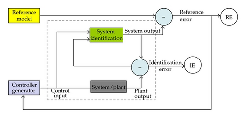
In the following, the whole control procedures are discussed in detailed computational expressions [41]. In the whole procedures, we usually identify the plant model first and then train the controller to make the plant output follow the reference model output.
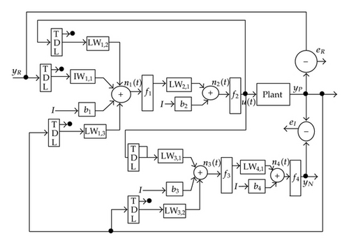
Here, we should emphasize that the reference model must provide the information which we desire for the plant output to follow. However, the reference model may or may not have any relation to the plant model. In economic control, we expect that the plant output with wide fluctuations can trace the desired reference output with approximate stable property in a high level.
3. Goodwin Growth Cycle Model
In this section, we will give a brief introduction of Goodwin growth cycle (GGC) model. GGC model [46] is a famous nonlinear economic model of the struggle between capital and labor for shares in national income, based on the classic Volterra-Lotka predator-prey model for populations. The control problem of original Goodwin model is not difficult to be solved, because some other important factors are not considered in the two-dimensional system, such as expected inflation rate. To show that our idea is very useful in solving the economic control problem, we will introduce a more complex Goodwin model in six dimensions.
The system (3.2)–(3.7) is very chaotic and has many unstable periodic orbits; see [47]. The time unit of this system is corresponding to the units of the variables. It is worth noting that the time unit should not be extremely small, such as second, minute and hour, for the rapid vibration is not acceptable in real economic systems. Here, we may let the time unit be a quarter, two quarters, or a year.
4. Application to GGC Model between Two Countries
In this section, we will apply MRC to the GGC model between two countries to demonstrate its validity. Our aim is to make the employment rate approximate stable in a high level by controlling the workers′ share in the national income. It shows that the control strategy is important for the policy maker. Here, we use the SIMULINK toolbox for SISO system in MATLAB (Version 7.0), which is designed by Hagan for controlling a robot arm [24].
The effect of MRC is great, if the trajectory of the reference model is very flat (in [21, 41, 42], the authors have all chosen the approximate stable systems to be the reference models). Also, our plant system (3.2)–(3.7) is chaotic as [42] has done. Hence, there is no doubt that this leads to good applicability of our work to use MRC in GGC model and its reference model. Here, the employment rate of the first country in the reference model (4.1)–(4.3) is approximate stable in 0.96, and this is an acceptable value in many countries or economic unions. So we choose (4.1)–(4.3) to be the reference model. Our main purpose is to control the employment rate of the first country in the plant to track along with the one in the reference model. In the following, we will show the main work of this paper.
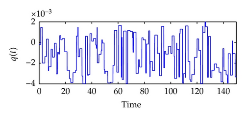
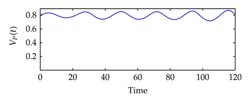
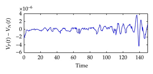
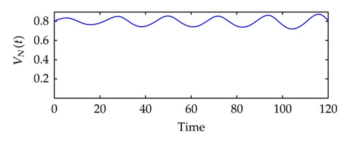
Next, we will train the network of system identification in q ∈ [−0.002, 0.004]. See Figure 5. Here, we use the Levenberg-Marquardt algorithm to construct a backpropagation neural network [48]. The built-in function of the algorithm in the SIMULINK is called trainlm. We use 300 training epochs for the system identification, and an epoch is just a recurrence of determining and adjusting the weights and functions in the layers through an error-minimizing process. From Figure 5(c), we can observe that the error v1(t)‒ v1N(t) is extremely small, and the real plant and the NN plant have almost the same outputs.
In the following, we will train the controller. It is more difficult to train a controller than to identify a plant, because the network here is recurrent and a dynamic backpropagation algorithm is needed. We will choose 13 segments for the training set and 10 epochs for each segment, and we will train the network of controller generation under the reference model input in r ∈ [−0.001,0.001]. See Figure 6.
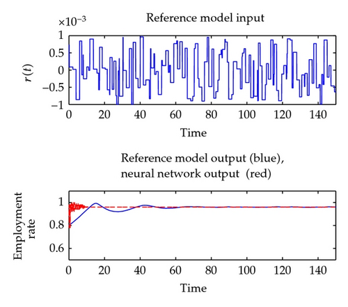
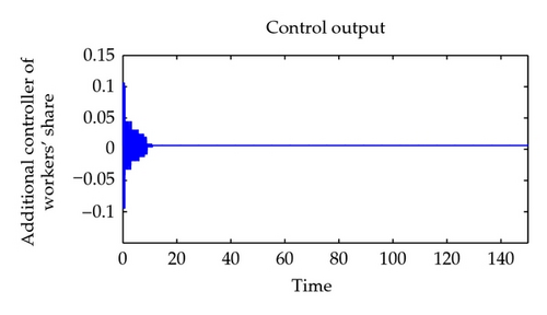
Now, the whole controlling process can be described as the following. The employment rate of the first country in the plant is widely fluctuant; however, the one in the reference model is approximate stable in long term. To drive the employment rate to follow the tendency of the reference model, one can adjust the workers′ share of the national income of the first country slightly. See Figure 8. The plant output is approximate stable at 0.96 in a long term, so our control effect is very remarkable.
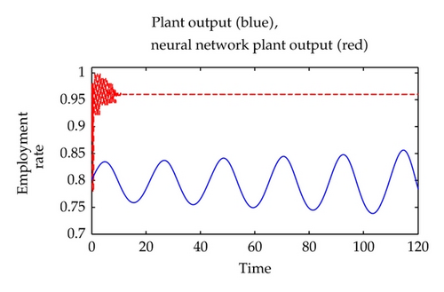
Though the two signals have nearly the same tendency, the signal after control is not tracking the signal from the reference model strictly. The reference model we used here is meaningful in economics, because it is obtained by driving the expected inflation rate of the first country to be zero, and has an approximate property in a high level by modifying a coefficient.
Obviously, a model with both simple tendency and suitable economic meaning might be better than our reference model. To make the reference model fit for the practical economic phenomenon, we still insist on choosing the model by driving the expected inflation rate to be zero. Indeed, the policy maker can constitute the fiscal and monetary policies according to the additional controller of workers′ share in Figure 7. The results show that we can control the workers′ share in the national income to make the employment rate approximate stable in a high level.
5. Conclusion
Model reference control technique has been used to control a complex economic system in this paper. The specific control method in engineering is very helpful to constitute economic policies for a country or an economic union. The simulation results show that one can control the employment rate stable in a high level by adjusting the workers′ share in the national income.
Acknowledgments
P. Zhao expresses sincere thanks to Professor Yong Li for his guidance, Professor Dayou Liu, and Professor Bo Yang for their instructions and many invaluable suggestions. Also, many thanks to the NSFC (Grant no.11071026, 11001100, 11171131, and 11026043) and the Basic Research Program of Jilin University (450060481098). This work is supported in part by the National Basic Research Program of China (973) under Grant 2009CB219301, the National Public Benefit Scientific Research Foundation of China under Grant 201011078, and the National Innovation Research Project for Exploration and Development of Oil Shale under Grant OSP-02 and OSR-02. The authors gratefully acknowledge the anonymous reviewers for their hard work and good patience.


