A Graph Approach to Observability in Physical Sparse Linear Systems
Abstract
A sparse linear system constitutes a valid model for a broad range of physical systems, such as electric power networks, industrial processes, control systems or traffic models. The physical magnitudes in those systems may be directly measured by means of sensor networks that, in conjunction with data obtained from contextual and boundary constraints, allow the estimation of the state of the systems. The term observability refers to the capability of estimating the state variables of a system based on the available information. In the case of linear systems, diffierent graphical approaches were developed to address this issue. In this paper a new unified graph based technique is proposed in order to determine the observability of a sparse linear physical system or, at least, a system that can be linearized after a first order derivative, using a given sensor set. A network associated to a linear equation system is introduced, which allows addressing and solving three related problems: the characterization of those cases for which algebraic and topological observability analysis return contradictory results; the characterization of a necessary and sufficient condition for topological observability; the determination of the maximum observable subsystem in case of unobservability. Two examples illustrate the developed techniques.
1. Introduction
The state variables that characterize a physical system are estimated by means of the data available at any given time. This data can be generated from a sensor network spread out over an area or from contextual and boundary constraints. In general, the known system variables are said to be sensed or measured variables whether they are sensed with a real device or their magnitudes are obtained in a sort of virtual sensors. The remaining variables are considered nonsensed or unmeasured variables. In such a context, the observability issue arises when we would like to know if the sensing system is enough to be able to determine the state of the system, that is, the system state variables.
This paper deals with a scenario where a well-known model describes the behavior of a physical system in terms of relationships between system variables and parameters. The system must be linear or linearized after a first-order derivative. In this context, a given sensing network is considered, and the system observability analysis is addressed.
The term observability was introduced in the realm of linear dynamical control systems [1]. It stems from the capability of estimating the state of a system based on the information available. Although observability is essentially a numerical and algebraic problem, some techniques based on topology and graph theory have been developed to provide solutions in this area.
Due to the fact that observability and the problems related to it were studied in different engineering disciplines, the technical terminology is not totally uniform. As a result, some terms are more widely used in some areas and not in others and, in a few cases, different terms describe the same thing in different fields.
Five examples are described below pursuing the following aims: on one hand, illustrating how observability and other related problems constitute research topics in different physical, engineering, and industrial areas, where a sensor network is designed in order to analyze a given system; on the other, showing the multiple points of view from which these issues can be addressed and, in particular, how topological and graph-based approaches were developed in some cases.
The term sensor network comprises a broad spectrum of engineering and physical systems and, in particular, the topic of wireless sensor networks has led to issues that, in one way or another, are related to observability. This is the case of coverage, optimal node placement, and the minimum number of nodes required to achieve connectivity. In [2], it is shown that a graph model can be used to describe those systems, and some graph approaches have been developed in order to provide an answer to the challenges posed.
Whithin the sphere of linear control systems, the controllability problem was addressed from a graph-theoretic approach. A graph associated to a system was defined in [3] and conclusions related to several system properties are derived from the analysis of such a graph. A survey of the techniques proposed in the literature for structured linear systems can be found in [4]. More recently, a graph approach to observability analysis is proposed in [5, 6].
High-voltage electric power networks constitute another field, where observability has been an important issue in system analysis for decades [7, 8]. It is worth mentioning that the approach to the problem in [9] where the authors characterize what they call topological observability through the existence of certain graphs that, defined in the electrical network, obey constraints derived from the sensing network. However, these graph techniques do not allow the inclusion of measurements that are currently being considered, such as current and phasor measures.
Observability has also been a motivation for research in traffic models in topics related to the origin/destination trip matrix estimation challenge. This is the case of [10], where the authors adapt topological techniques developed for electric power networks to this new context. Although this issue is more complex than the description made by the authors in their paper, it has been taken as an example to illustrate the techniques proposed in the present work as will be shown in a later section.
Material and energy balances that must take place in industrial processes are analyzed in [11]. There, its authors distinguish up to four categories of balancing equations, depending on whether they consider or not materials, chemical reactions, energy, and entropy. They study the solvability of the resulting equations, for which a set of sensed variables is taken into account. The observability and redundancy of measurements as well as the errors in the measured values are included in the dissertation. Statistical techniques are used to estimate the state of the system by reconciliation. In the case of linear systems, a parallelism is established between system and sensing observability conditions and the existence of certain graphs defined from the process balancing flowsheet.
The common topic of the aforementioned scenarios, with regards to graph theory, is that certain graph techniques were developed in all the cases because of the existence of graphs or networks that characterized the systems with a given sensor set. Furthermore, the equations that describe the networks are linear or linearized. In this paper, a new graph technique is presented in order to characterize the observability of any linear physical system. The implementation of such a technique imposes constraints on the problem, summarized by the fact that the systems must be sparse and of large dimension. For any sparse and large dimensional physical system, an associated network will be defined based, exclusively, on structural considerations, that is, the topology of the equation system in its matrix form that relates the sensed variables with the state variables. It will be demonstrated that the system can be said to be topologically observable if there exists a certain graph within the associated network.
Krumpholz et al. developed in [9] a topological approach for the observability issue in the scope of electric power systems. Nevertheless, the problem related to the characterization of those cases for which algebraic and structural techniques return contradictory results is not studied. In this paper, the latter problem is solved, which has allowed carrying out a more general demonstration of the necessary and sufficient condition for topological observability than the one proposed by Krumpholz. Numerous techniques have been developed and widely and successfully tested for decades [12–15] in the scope of topological observability analysis in electric power systems. In this paper, a new graph approach is presented, which allows addressing the observability of any linear physical system or, at least, a system linearized after a first-order derivative, and not exclusively electric power systems. Boukhobza et al. had already developed a graph-theoretic technique in order to determine the state and input observability in structured linear systems [5]. Unlike that proposal, the approach presented in this paper makes it possible to exploit techniques like those mentioned above [12–15] to characterize concepts like parametric unobservability and to easily determine the maximum observable subsystem.
The rest of the paper is organized as follows. Starting from a mathematical model, some terms will be introduced concerning observability and sparse physical systems in the next section. Section 3 is devoted to the bases of graph theory and the concepts used throughout the paper. Once the theoretical assumptions have been described, an analogy between linear equation systems and graph theory is established by means of a network associated to the physical system and a given sensor set. Section 5 introduces the concept of topological observability, which is characterized through the existence of a constrained graph in the associated network. The following section is devoted to the cases where the system is not observable and how the search for the maximum observable subsystem is addressed by means of the same graph techniques. Section 7 includes two examples in order to illustrate the techniques proposed in this paper, and how they can be implemented in absolutely different real engineering scenarios. Finally, some conclusions are presented in Section 8.
2. Mathematical Model
Let S be an n-dimensional physical system that is going to be the object of our study, and let a sensed variables set z be defined, where m magnitudes are measured over S. Furthermore, let M be the m × n matrix associated to S, as defined in (2.4). We will say that S is a sparse system if the behavior of S at any point can be justified exclusively by means of the knowledge of the variables in an area based on a certain neighborhood relationship. This is the case of a traffic model system where flow fluctuations in a certain region are strongly dependent on what happens in that area, whereas the events that take place in other parts show a weak dependence or absolute independence from them. One of the features that characterize a sparse system is that matrix M is a sparse matrix. Then, some conclusions can be established in terms of structural considerations of M, when the matrix dimensions and the degree of sparsity are large enough. For this purpose, Bunch and Rose [21] define a graph associated to a matrix M, where a nonzero element mij ≠ 0 of M represents an edge that joins vertices i and j. Based on this, some properties can be studied in terms of graph theory because of the duality between sparse linear systems and graphs.
The obvious solution of calculating the rank of matrix M may present problems and may not be even possible in the case of ill-conditioned systems, as mentioned above. In these cases, a topological-based approach becomes a good choice that presents a series of additional advantages derived from the capability of graphs to answer questions related to observability analysis, including the identification of the maximum observable subsystem and optimal additional sensor placement. In short, in this paper we will introduce new topological analysis techniques by means of certain graphs associated with sparse systems in order to determine the topological observability of such systems.
3. Graph Theory
A graph is defined as a collection of nodes or vertices that are joined through the so-called edges or branches. For the sake of homogeneity here we will use the term branches both for general graphs and for the case of trees, which are basically graphs without loops. In the scope of this work we are interested in defining graphs within a given network, which is also a collection of nodes and branches. In other words, a network must be interpreted as the context where any given graph is declared, in such a way that nodes and branches belonging to a graph are also present in the network for which the graph is defined. Nevertheless, not all the nodes and branches of the network are always present in a graph.
Definition 3.1. Let X = {X0, X1} be a network, where X0 and X1 are the sets of nodes and branches, respectively; a graph G of X is defined as a set of nodes, G0⊆X0, and a set of branches, G1⊆X1.
Definition 3.2. A graph T of X is said to be a spanning tree if T contains no loops, and T0 = X0.
A directed graph results from the assignment of a direction to each branch in such a way that a node is known as the source, while another node is the target of a directed link.
Definition 3.3. Let X be a connected network, a graph G of X is said to be of full rank if its rank equals the maximum possible value, rank {G} = size{X0} − 1.
Definition 3.4. The closure [22] of a connected graph G in X is defined as a graph , where and is composed by all the branches in X1 that join pairs of nodes in G0.
4. Network Flow Analogy
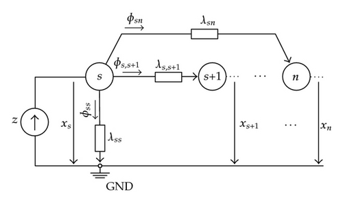
Note that, on one hand, the elementary network in Figure 1 is characterized by the nodal (4.3), where the flow injected in node s equals the z magnitude; on the other hand, a solution {xs, …, xn} to the elementary network in Figure 1 is consistent with (4.1).
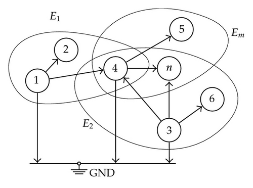
Equation (4.7) characterizes network X as well as (4.8) characterizes system S from a set of variables {z1, …, zm} and, therefore, from equalities (4.7) and (4.10) it can be concluded that the study of the determinism of S is equivalent to the observability of X under constraints related to the variables zk taken into account.
5. Topological Observability
Krumpholz et al. introduced in [9] the term parametric unobservability as a vague notion needed to justify the concept of topological observability in electric power networks under certain assumptions. In this section, we present a formal description that allows defining and characterizing parametric unobservability and demonstrates how topological observability can be addressed by means of the existence of certain graphs under constraints.
Let S be a large n-dimensional sparse physical system, where a sensing system z is defined by means of m measured variables, m ≥ n. Let M be the coefficient matrix, as defined in (4.8), associated to S and the sensing system, and let X be the associated network. It is important to note that M characterizes only those parts of the system related to measurements, but not the whole physical system. In particular, it shows the relationship between the sensor set considered and the state variables. Therefore, M might be a diagonal or block diagonal matrix, without implying either the existence or nonexistence of decoupled subsystems in S. Obviously, the observability analysis of decoupled subsystems, if they exist, can be carried out independently.
It is clear that the first entry in Mn in the first row is nonnull and, therefore, there exists in Xn a branch joining node 1 and the reference node. In the second row, there are two possible cases: on one hand, if the diagonal element is the first nonzero element in that row, there exists a branch in Xn joining node 2 and the reference node and, indirectly, the first node too; on the other hand, if the diagonal element is not the first nonzero one, there is a link in Xn between nodes 2 and 1. This argument can be repeated for the next row and up to the last one. Eventually, a spanning tree of full-rank T of Xn is completed because of the lack of loops and the inclusion of the totality of the nodes in the network. Furthermore, the previous analysis leads exclusively to one branch in T from each row in Mn. In other words, the n branches in T are derived from n different measurements in z. Since Xn results from the superposition of n elementary networks, one for each sensed value, each branch in T belongs to a different elementary network.
In order to demonstrate that the existence of such a spanning tree is sufficient, under certain conditions, for the observability of a system with respect to a sensing configuration, a reverse path is considered in which branches are added recursively to a starting spanning tree until the entire network is encompassed.
- (1)
the additional branch a joins node s and the reference one. Therefore, as the admittance of this branch is equal to , the only entry that makes matrices M(T) and M(T+1) different is:
()and, from (5.5), the determinant:()that is equal to zero when:() - (2)
the additional branch a joins node s and a node j, where s < j ≤ n. In this case, the branch admittance equals λa = −αkj and both matrices M(T), and M(T+1) are equal but for two entries in row k:
()and, again, the determinant:()that vanishes when:()
- (1)
the additional branch a joins nodes s and the reference one. The admittance of branch a is equal to and the determinant of M(T+r+1) is estimated by:
()where is the cofactor of . The above determinant becomes null when:() - (2)
the additional branch a joins node s and a node j, where s < j ≤ n. Then, the branch admittance is equal to λa = −αkj, and the determinant of M(T+r+1) is given by:
()where and are the cofactors of and , respectively. The determinant will be null if:()
Note that (5.13) and (5.15) allow identifying a set of values of coefficients αki for which the determinant |M(T+r+1)| might be canceled.
New branches can be added to the given graph, one by one, until the entire network Xn is completed, after the inclusion of all the branches in Xn. Therefore, it is concluded by induction that the determinant of matrix M(Xn) is nonzero if its entries αki, 1 ≤ k, i ≤ n, do not meet any equality such as (5.8) and (5.13) for branches that join the reference node and (5.11) and (5.15) otherwise.
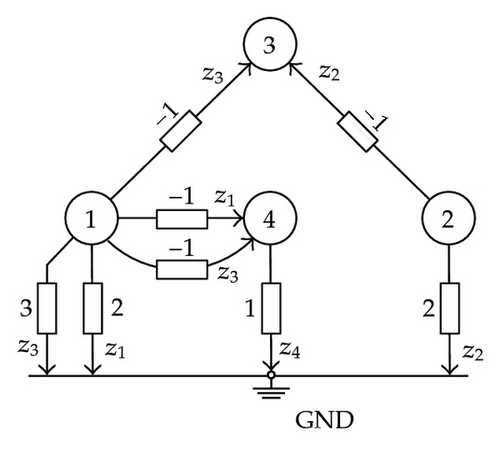
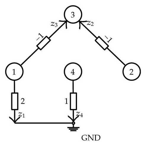
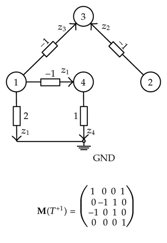
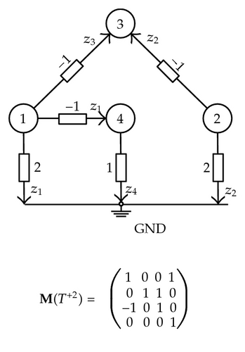
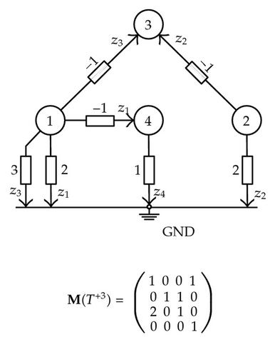
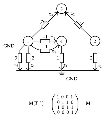
Note that this result was reached from the consideration of, on one hand, the network topology and the number, nature, and location of sensors in the network and, on the other, the network parameters. To deal with these two approaches, the concept of parametric unobservability is introduced.
Definition 5.1. A large dimensional and sparse physical system S, for which a sensing system z is defined, is said to be parametrically unobservable with respect to z if, in spite of the fact that the ranks of matrices B(X) and YA(X) are equal to n, the rank of M is less than n due to the value of one or more coefficients αki of M.
The relevance of this concept lies in the fact that, in large dimensional sparse physical systems where the parameters are roughly estimated from empirical data or are subject to environmental distortion, it is unlikely for parametric unobservability to occur [9]. In other fields, such as structured linear systems, it is often necessary to work under the assumption of a lack of knowledge of system parameters [4]. In these scenarios, the parametrically unobservability should be associated with a particular set of parameter values. Thus, the observability of a system is said to be true when it is so for almost all parameter values, that is, for all of them except for a set of particular cases in the parameter space. Even though not all physical systems may meet this requirements, there exist evidences that are true for real cases. For example, electric power network analysis involves hundreds or even thousands of state variables that are usually related to the voltage at network nodes. The system state [7] can be estimated by means of the measurement of the power that flows into and through the electric network and which is influenced only by neighboring node states. Thus, the resulting system is clearly sparse, and circuit parameters are affected by environmental conditions such as temperature and humidity as well as by the unreliability of parameter estimation. Another example is the case of traffic model analysis [10]. As explained later in the example in this paper, vehicles usually move along a geographical area according to a set of established origin/destination pairs. Traffic flows are sensed at routes in the network in order to estimate the state of the system, that is, origin/destination pair traffic flows. As the network grows, the sparsity becomes more plausible. Additionally, system coefficients are estimated, among other factors, from probabilistic considerations related to the ability of people to opt for one route or another. In brief, parametric unobservability is, in these two cases, highly improbable despite being mathematically possible.
On the basis of the large dimension, sparsity and parameterization uncertainty of such systems, in order to address the observability issue a new strategy is proposed involving exclusively structural and not numerical considerations. For this, a new observability definition should be provided.
Definition 5.2. Let S be a large dimensional sparse physical system, where a sensor network z is considered; S with z is said to be topologically observable if S is algebraically observable or parametrically unobservable with respect to z.
Summarizing, it has been demonstrated that the existence of a spanning tree of full-rank T of X where the n branches of T belong to n different elementary networks of X constitutes a necessary and sufficient condition for topological observability. In what follows, any graph G of X with a number rG of branches that belong to rG different elementary networks, that is, are associated to rG different measurements zk of z, is known as a measured graph.
Theorem 5.3. Let S be a linear and large n-dimensional sparse physical system, where a sensing system z is defined by means of a number of m measured variables, m ≥ n; S is said to be topologically observable with respect to z if and only if there exists a measured spanning tree T of X.
The analysis of the observability of a large dimensional sparse physical system S with respect to a sensing system z from a topological point of view involves searching for a measured spanning tree T of full rank among all possible graphs G of X constructed in such a way that each elementary network that forms X contributes with and only with one branch to G. If the number of sensed values m considered is larger than the dimension n of system S, T will be included, if it exists, as part of a measured spanning graph G of X. In what follows, it is assumed that any graph G of X is a measured graph.
There could be different ways to construct a spanning tree, and any one of them would be valid [12–15]. However what is important here is the fact that the existence of a measured spanning tree is a sufficient condition for the topological observability of a linear system.
Summarizing, taking as a basis the experience in observability analysis in electric power systems, a generalization of the topological approach was developed to address this issue in the scope of other linear, or linearized after a first order derivative, real engineering physical systems. A necessary and sufficient condition for topological observability was established by means of a graph theoretic approach. Finally, thanks to this approach, the characterization of the cases where algebraic strategies do not lead to the same results as those derived from structural analysis was carried out.
6. Maximum Observable Subsystem and Observability Islands
If the observability system test fails for a sensing configuration, it is said that the system is not observable or unobservable. In such cases, the knowledge that might be acquired about one or more parts of the system by all the measures considered should not be underestimated. If a system is not observable, it may be possible to identify a subsystem for which the state can be estimated, it is said that the subsystem is observable. A nondivisible observable subsystem is known as an observability island. The number of observability islands may vary and depends on the associated network topology, the sensors considered and their location in the network.
Consider an n-dimensional sparse physical system S and a sensing configuration z for which an associated network X is defined. Let O be an observable island of S and z, and let XO⊆X be its associated subnetwork; XO is known as an observable subnetwork.
A node belonging to XO is said to be an observable node, and a branch belonging to XO is an observable branch. A measured spanning graph G of XO is known as an observable graph. Nodes and branches that do not belong to any observable subnetwork are said to be unobservable.
Let Y be a measured graph of X; a measure zk associated to a branch of Y is said to be wholly contained [22] in Y if the elementary network associated to zk is contained in the closure of Y in X. By extension, a measure is said to be wholly contained in a subnetwork XO if its associated elementary network is included in the closure of XO in X.
Any measurement zk considered in O is wholly contained in XO. Hence, the state of an observability island may be estimated by means of a wholly contained sensor set.
The union of all the observability islands in a system S derives in a maximum observable subsystem while the union of all their associated observable subnetworks in X results in the maximum observable subnetwork. This subnetwork is maximum because it comprises the largest possible number of observable nodes and, if it exists, it is unique [22].
Consider a system S that is not observable for a sensor set z. Then, no measured spanning tree will be found, as derived from Theorem 5.3. Instead, consider a measured graph G of X as one of the largest connected graphs that can be formed according to the sensing system and the constraints described earlier. Then, G is known as a maximum measured graph of X but not spanning. The next theorem was extracted from [22], where relevant properties concerning maximum measured graphs and observable subsystems are described.
Theorem 6.1. Let S be a system and X the associated network from a given sensor set. If G is any maximum measured graph of X, the maximum observable subnetwork is contained in the closure of G in X.
Therefore, based on one of the maximum measured graphs, an iterative process can take place by which the not wholly contained measurements, and their elementary networks are removed from the system until the maximum observable subnetwork is obtained. Additionally, other strategies concerning the search for the maximum observable subsystem can be found in [13, 14] in the scope of electric power networks.
7. Examples
Two examples are presented in this section in order to illustrate the techniques developed in this paper, focusing the attention on the fact that these techniques are valid for different real engineering problems, where a collection of linear equations or equations linearized after a first order derivative describe the behavior of the system from a measurement acquisition system viewpoint.
7.1. Traffic Model Example
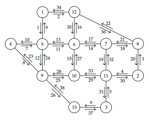
Figure 5 shows a benchmark case, known as the Nguyen-Dupuis network [23] in the literature, consisting of 13 plausible origin/destination places that are interconnected by 19 bidirectional links. In that scenario, vehicles can move from one place to another through suitable routes. Figure 5 shows indices assigned to links along with their directions. Therefore, for an OD-pair, any possible path is defined as a series of oriented link indices; for example, the sequence {2,36,20} denotes an alternative for a displacement from 1 (origin) to 2 (destination).
7.1.1. Case 1: Observable Configuration
The question arises as to whether OD-pair traffic flows x can be estimated from this sensor set z among the aforementioned oriented link flows.
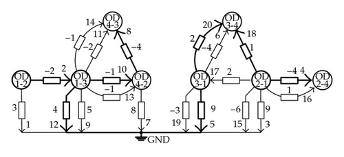
In Figure 6, the elementary networks derived from the coefficient matrix M of (7.4) are shown. Note how OD-pairs play the role of network nodes, while OD-pair traffic flows are the network node potential levels. In the figures, branch admittance values are indicated; indices were assigned to the branches and are shown in the figures by smaller numbers next to the arrows.
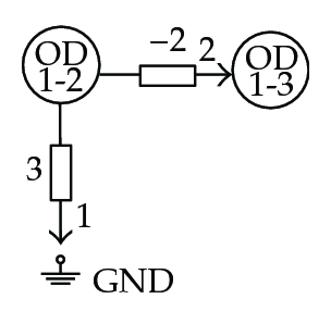
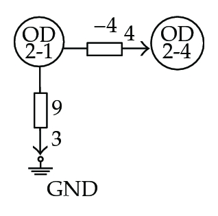
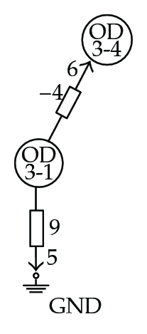
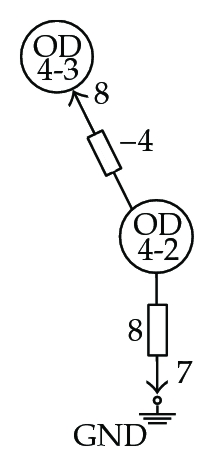
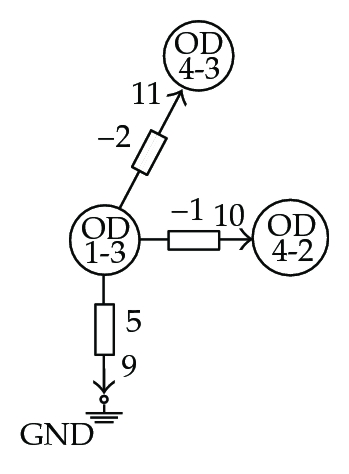
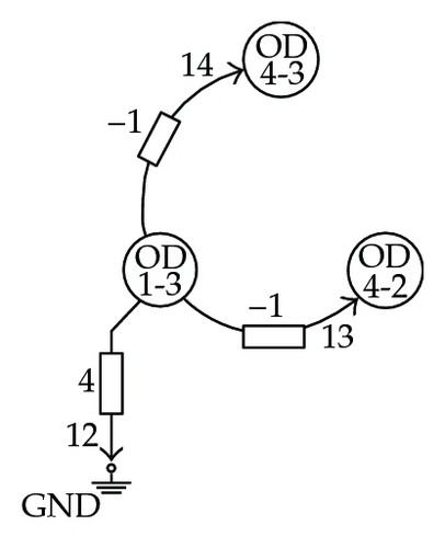
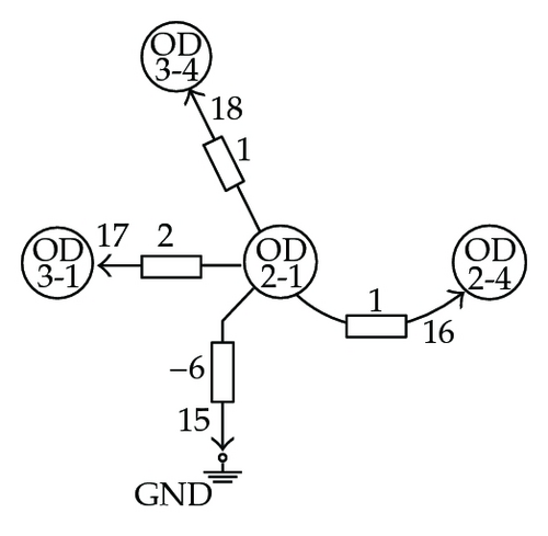
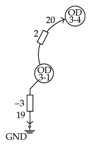
Figure 7 shows the entire associated network and how a measured spanning tree, highlighted using thick line, was found among other possibilities. Note that each elementary network is related to one and only one branch in the resulting measured spanning tree. This tree is not unique but the existence of, at least one, guarantees the topological observability of the system for the sensor set defined in (7.4).
7.1.2. Case 2: Not Observable Configuration
In a second case, a total of 6 traffic flow meters are considered. The question arises as to whether system observability can be achieved by incorporating additional sensors. And if it is not possible, which is the maximum observable subsystem?
Figure 8 shows the resulting associated network, X, and one of the possible maximum measured graphs, G (thick lines). Note that OD-pairs 2-4 and 4-3 are clearly not observable, that is, their traffic flows cannot be estimated by means of the available measurements. A more detailed analysis leads to the conclusion that measurements v4, v7, and v12 are not wholly contained in G and, therefore, their associated elementary networks E2, E4, and E5, respectively, should be removed from the network in order to search for the maximum observable subnetwork. This argument should be repeated until the resulting subnetwork is made up exclusively of elementary networks associated to wholly contained measurements. That is the case after removing E1, the elementary network associated to measure v2. From there, the maximum observable traffic subsystem is immediate and is given by OD-pairs 3-1 and 3-4 and oriented traffic link flow sensed values {v5, v38}.
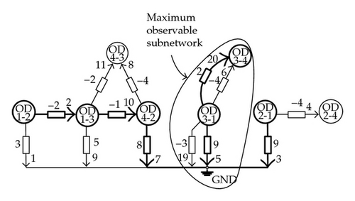
that allow joining OD-pair 4-3 node, would permit observing the whole traffic system.
7.2. Electric Power System Example
As it was mentioned in the introduction, observability analysis in electric power systems has been an important research topic for decades. In particular, this issue can be addressed by means of topological methods, when the set of measured variables are made up exclusively of bus voltages and active and reactive powers that are injected into or flow through the system [9]. In those cases the system can be considered as a decoupled system [7], that is, a pair of two independent subsystems: one of which can be analyzed by means of active power measurements, and is known as P-δ subsystem; the other one, the Q-U subsystem, can be studied exclusively from bus voltages and reactive powers measured in the system. Only the Q-U subsystem is going to be analyzed in this example. Such a subsystem is observable [7] when a sufficient number of well-placed reactive powers are measured, and, at least, one node voltage is known at any node.
- (i)
node measurements, numbered as 1, 2, and 3 in Figure 9(b), corresponding to reactive powers injected into the system through a node. These derive in equations of the form:
()where Qi denotes the i-th node reactive power, Ui represents the voltage at node i, αki is a coefficient related to measurement k and node i, and ck denotes a constant term related to measurement k; - (ii)
branch measurements, numbered as 4, 5, 6, and 7 in Figure 9(b), corresponding to reactive powers that flow through the lines. These derive in equations of the form:
()where Qij denotes a branch reactive power that is acquired in a line that joins nodes i and j.
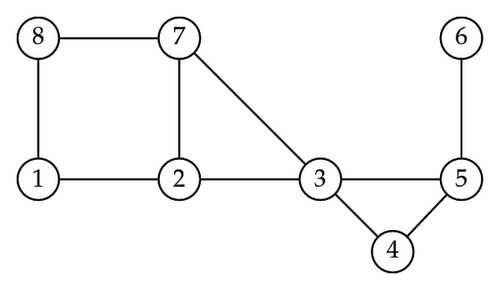
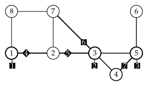
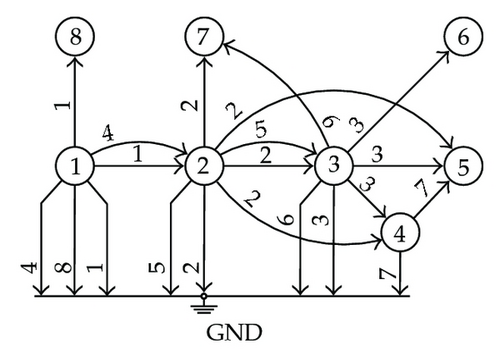
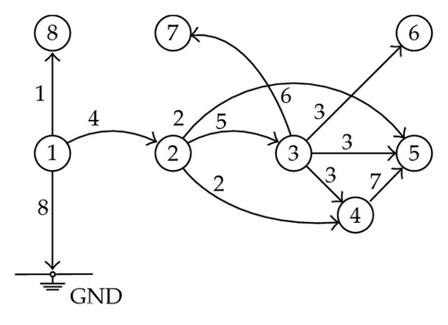
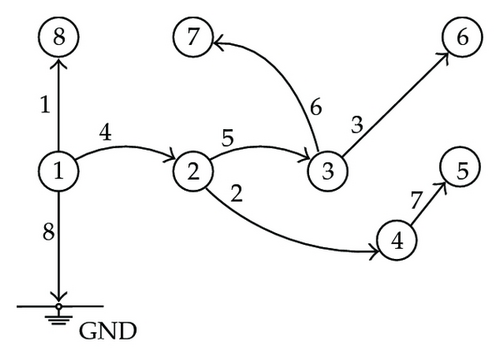
Finally, one of the possible measured spanning trees is shown in Figure 9(e), after the assignment of each of the eight measurements considered to one of the edges in the associated network. The existence of such a tree permits concluding that the electric power Q-U subsystem is topologically observable for the given sensing system.
8. Conclusions
In this paper, a new topological approach to the determination of the observability of a physical system where a sensor network is defined has been presented. The techniques developed in this paper were inspired by the contributions of researchers in the scope of electric power systems and generalized to other physical sparse linear systems. The terms parametric unobservability and topological observability have been introduced and justified in a formal way, which allows characterizing those parameter dependent cases where an algebraic approach to the observability issue led to different results than the topological one. A sensing system has been considered for any linear physical system or, at least, linearized after a first order derivative. From there, an associated network has been defined, and it has been demonstrated that the existence of certain constrained graphs, known as measured graphs, in the scope of the associated network permits characterizing the topological observability of the system. From this graph approach, the determination of the maximum observable subsystem can be carried out in case of unobservability. The technique has been illustrated with the help of two examples in the scope of traffic sensing structures and electric power systems.
Acknowledgments
This work was partially funded by the Xunta de Galicia, the MICINN of Spain and European Regional Development Funds through projects 09DPI012166PR, 10DPI005CT, and TIN2011-28753-C02-01.


