On Three Competing Maintenance Actions and the Related Condition Control
Abstract
This paper considers three competing maintenance actions: corrective after failure, condition-based preventive to avoid failure, and scheduled. A stochastic model is set for the time relationship between corrective and preventive maintenance. This model defines a version of the so-called random signs censoring, and it leads to natural goodness measures for condition control. The effect of condition control on important observable and unobservable indicators is studied. The latter half of the paper considers static Weibull models for the time to failure and the effect of condition control; the main contribution is a calculation method that derives the four model parameters from four figures of input data. Corresponding parameter experimentation is demonstrated on maintenance cost analysis and condition control design.
1. Introduction
Since some decades, competing risks models have been employed and further developed in the reliability field. The notion “random signs censoring” [1] is well established, and different refinements have been introduced, for example, the “repair alert model” [2]. The repair alert model again has been modified further, for example, to incorporate opportunistic maintenance [3]. Cooke’s [4] claim for “more models of dependent competing risks in which critical failure probability is identifiable” applies to this paper, too. For broader information about the state of art, we refer to [3, 4].
Our basic tool is an independent random variable S that represents the condition control system in two ways. First, a combination of S and the unknown time X to failure models the condition-based planned time to preventive maintenance; this model defines a random signs censoring, but it is not a repair alert model. Second, in terms of S, we also define natural measures for the effect of condition control: trustworthiness, exactness, and general goodness. Thereafter, we study some indicators (probabilities and means) as functions of S, X, and the time H to next scheduled maintenance—especially their relation to trustworthiness and exactness.
In the latter half of the paper, we add three assumptions frequently used in case studies. We develop an analytic-numeric method, where the output is two-parameter Weibull models for S and X and the input consists of four single figures, that is, values of indicators assessed from field data or presumed for new design. For comparison, many existing methods make use of the empirical subsurvival functions, which require quite detailed input data [5]. Then, the models obtained for S and X act as the centre of parameter experimentation. We analyse the maintenance-related long-term costs as a function of H, and we study the requirements to be put on the condition control in order to achieve specified improvements of the indicators.
The last section shortly declares a motive for extension.
2. Three Competing Maintenance Actions
- CM
If a failure (critical failure) occurs, it interrupts the task execution and corrective maintenance must be performed.
- PM
The condition control system (maintenance crew included) proposes a time instant for preventive maintenance to avoid failure and CM.
- SM
Regardless of the component’s condition, there is a planned time point for next scheduled maintenance.
-
X unknown time to failure and CM,
-
Y decided condition-based time to PM,
-
H planned time to next SM (H = ∞ if there is no SM plan).
Now, the least member of the triplet (X, Y, H) determines the type and the time instant of the maintenance action that terminates the service sojourn (Table 1).
| If condition | Time to maintenance | Terminating action |
|---|---|---|
| X < Y & X < H | X | CM |
| Y ≤ X & Y < H | Y | PM |
| H ≤ X & H ≤ Y | H | SM |
Let us immediately interpret some orderings of X, Y, and H. (a) If X < H ≤ Y, then a failure (CM) ended the sojourn and PM was not planned at all. (b) If X < Y < H, a PM action was planned but in fact unnecessarily, since a failure (CM) came earlier. (c) If Y < H ≤ X, PM was performed but in fact unnecessarily, since SM would have saved the component from failure. (d) If Y ≤ X < H, the performed PM really saved the component from failure.
Generally taken, the spans X, Y, and H can depend dynamically on component age, maintenance history, environment, physical conditions, strategies, and so forth. We exemplify here with such SM schedules where the actions are fixed in advance on the time axis: if the ith sojourn terminated with a CM, that is, Xi < Yi & Xi < Hi, then the time to next SM is Hi+1 = Hi − Xi, and if it terminated with a PM, that is, Yi ≤ Xi & Yi < Hi, then Hi+1 = Hi − Yi.
3. Basic Models and Concepts
3.1. Condition-Based Time to Preventive Maintenance
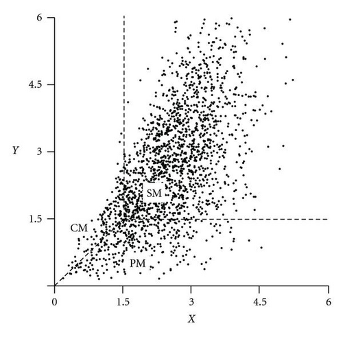
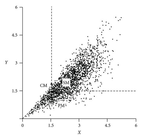
Figure 1 illustrates how the point (X, Y) defined by (1) hits one of the xy-regions CM, PM, or SM, according to Table 1. The right-hand case depicts the “better” control system, since Y < X more often and Y/X is closer to 1. Section 3.2 provides exact definitions.
3.2. Goodness of Condition Control
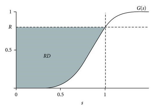
Verbally expressed, trustworthiness is the probability that PM saves the component from failure and exactness is the expectation of the ratio Y/X given that PM saves the component from failure. Indeed, (1) implies Pr(Y ≤ X∣X < H) = Pr(Y ≤ X) = R and E(Y/X∣Y ≤ X < H) = E(Y/X∣Y ≤ X) = D for all H > 0. Further, both R and D dwell in the unit interval with “bad” values near 0 and “good” values near 1, so RD describes the general goodness of condition control. Figure 2 illustrates the measures R, D, and RD.
3.3. Indicators for Applications
We clarify some immediate relations to the condition control. Good trustworthiness (R) means low probabilities of failure (κc) and unnecessarily planned PM (K), because K ≤ κc ≤ 1 − R (by definitions). Good exactness (D) again leads to low probability of unnecessarily performed PM (L).
To justify the last statement, consider a sequence Sn with cumulative distributions Gn(s), n = 1,2…, such that the exactness Dn → 1 (3). We state that Gn(s) → 0 for every s ∈ (0,1) or, equivalently, Gn(H/x) → 0 for every x > H. (If this were not true, there would be an s′ ∈ (0,1) and a δ > 0 such that Gi(s′) > δ for all i in an infinite set of positive integers, but this brings the contradiction Di < 1 − (1 − s′)δ for all i). Now, pick any ε > 0 and let a > H be such that 1 − F(a) < ε/2. The Lebesgue convergence theorem [6, Page 229] says that there is an integer nε > 0 such that . Hence, Ln ≤ A + 1 − F(a) < ε, for n > nε. Since ε was arbitrary, we have Ln → 0.
4. Static Models for Time to Failure and Condition Control
4.1. Additional Assumptions and the Main Problem
- (i)
The time-to-failure distribution F(x) is the same for every sojourn; that is, every CM, PM, and SM restores the component to the same condition.
- (ii)
The distribution G(s) is the same for every sojourn; that is, the relevant properties of the condition control do not change from sojourn to sojourn.
- (iii)
The planned time H to next SM is the same for every sojourn. (This means of course that the SM schedule moves forward after every CM and PM.)
4.2. Solution of 4′ and 5′
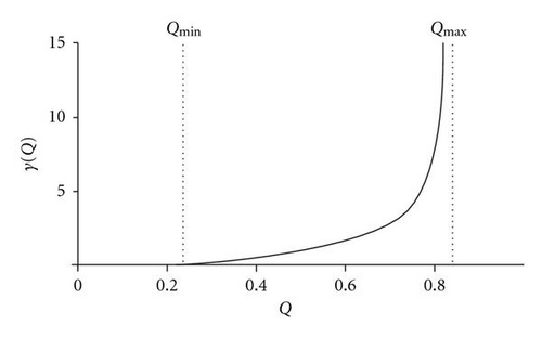
These facts imply that A(Q, 0)< κp<A(Q, ∞) if and only if Qmin < Q < Qmax . Because of continuity, there is for each Q in the interval (15) a positive number γ = γ(Q) satisfying (14) and for other Q there are no γ. In addition, by partial differentiation, one finds that A(Q, γ) is increasing as a function of γ for each Q in (κc, 1) and decreasing as a function of Q for each γ > 0. This monotony settles some facts: γ(Q) is unique and increasing and the triplets (Q, γ(Q), P(Q)) form the solutions of (4′) and (5′).
Figure 3 collects the results of the numerical example (Section 4.1): Qmin = 0.238095, Qmax = 0.840000, and γ(Q) calculated for 200 equidistant Q-values.
4.3. Solution of (6′) and (7′)
Figure 4 depicts the results of the numerical example (Section 4.1): Pmin = 0.790000, Pmax = 0.940476, and α(P) calculated for 200 equidistant P-values.

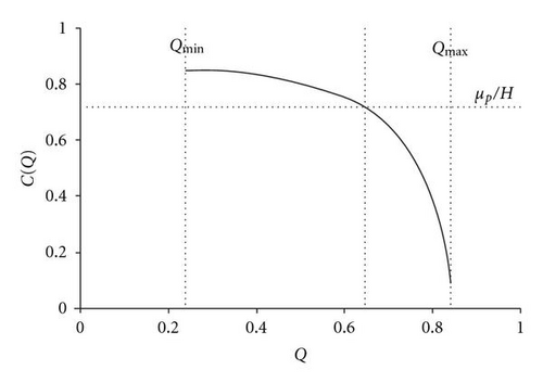
Figure 5 depicts the results of the numerical example (Section 4.1): C(Q) calculated for 200 equidistant Q-values and the solution Q = 0.6449 of (18).
4.4. Results and Comments
The solution Q of (18) determines now the other parameters: P = P(Q), γ = γ(Q), α = α(P), and β = α/γ. Insertion of the parameters P, α, Q, and β in (11) and (12) yields the time-to-failure distribution F(x) and the condition control representative G(s). The numerical values of the example (Section 4.1) are depicted in Table 2.
| Parameters | P = 0.9225 | α = 5.7909 | Q = 0.6449 | β = 3.0263 (γ = 1.9135 = α/β) | |
|---|---|---|---|---|---|
| Sojourn | Fraction check | Average length check | |||
| CM | Q(1 − P) = 5.0000% | κc = 5% | B(P, α) = 0.850000H | μc = 0.85H | |
| PM | A(Q, γ) = 16.0003% | κp = 16% | C(Q) = 0.720002H | μp = 0.72H | |
Remark 1. The calculation method in Section 4.2–4.4 lends itself for relatively simple and reliable computation, especially because of the stepwise structure and the monotony of certain functions mentioned above. The solutions of (14) and (16), γ(Q) and α(P), were iterated for 200 equidistant values of the variables in their respective domains, and linear interpolation was used for intermediate values. The software to be employed for accurate programming may readily offer built-in equation solving, numerical integration, and simple programming tools.
Remark 2. The input quadruplet (κc, κp, μc, μp) led to the output quadruplet (P, α, Q, β). However, the same tools also apply to certain mixed input quadruplets, for example, (κc, κp, α, β), (κc, κp, P, α), (κc, κp, P, β), (κc, κp, Q, α), and (κc, κp, Q, β). Indeed, check the consistency of the input in (10), (15), and (17) and then apply (6), (7), (13), (14), and the relation α = βγ in suitable order to get the remaining unknowns.
5. Parameter Experimentation
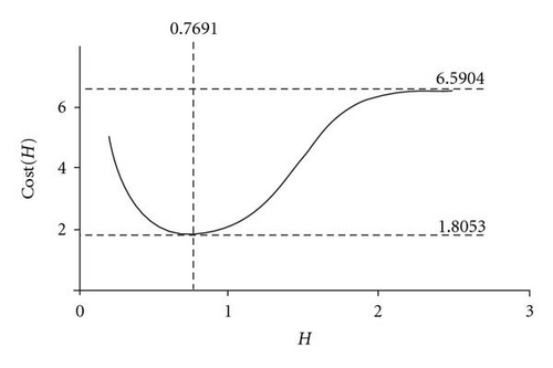
Example 1. We look at the maintenance-related costs as a function of H, while the component (P, α) and the condition control (Q, β) stay unchanged. Suppose that the costs for different maintenance actions are proportionally D = 1 per SM, Dc = 10 per CM, Dp = 4 per PM, and Dp0 = 1 per unnecessarily planned PM (8). (These costs can include work, spare parts, facilities, lost revenue, penalties, etc.) The indicators (4)–(8) are functions of H only, so the long-term maintenance-related cost per unit execution time is given by
Example 2. We analyse the effect of the condition control (Q, β) while (P, α) and H = 1 stay fixed. Suppose that we want the probability of failure down from the present κc = F(1)Q = 5% to 3%, (4). Clearly, this requires that Q = 0.6449 · 3/5 = 0.3869. Because of this change, the probability of unnecessarily performed PM (9) increases from L = 0.132 to 0.258, but suppose that we want L = 0.100. By solving (9), we get the required β = 7.0871. Moreover, according to Table 3, the required changes (κc = 5% → 3% and L = 0.132 → 0.100) correspond to improving the trustworthiness from R = 0.3551 to 0.6131 and the exactness from D = 0.7280 to 0.8481. In fact, this correspondence is always valid, since there is a continuous bijection between the pairs (R, D) and (Q, β).
6. A Motive for Extension
Discrete event simulation is the superior alternative for modelling complex real-world processes over long periods [7, Page 2–4], and the related field of random variate generation provides the modeller with an enormous variety of algorithms, (e.g., [8]). Generalizations, extensions, ex tempore decisions, and other intricate details are much easier to model in a proper stochastic simulation environment than in an analytic formulation. An imperative benefit, for example, for persuasive cost and risk accounting, is the output of various complete probability distributions (instead of “means”).
These facts among many motivate developing our concepts towards dynamic simulation. The constellation and the tools of Sections 2 and 3 are applicable as such, but Sections 4 and 5 deal with static models only. Let us sketch a first step, where the time X to next failure (and CM) can depend on the component’s age t (cumulated execution time) at the sojourn start. Now, the distribution of X could be, for example, of the type F(x∣t, α) = 1 − eΛ(t,α)−Λ(t+x,α) that generates a nonhomogenous Poisson failure process with cumulative rate Λ(t, α). The model parameter(s) α can be maximum likelihood estimated from typical field data consisting of consecutive sojourns where PMs and SMs are right-censored CMs.


