A Comparative Study of VaR Estimation for Structured Products
Abstract
The previous literature commonly concluded that GARCH models provide better volatility forecasts in financial markets. This paper adopts the backtesting criteria, the multivariate extension of the Diebold and Mariano (1995) test, RMSE (root mean squared errors), and MAE (mean absolute errors) to compare the performances of selected conditional heteroscedastic models for structured products in the low oil price and high oil price periods. The results illustrate that, in general, the performance of GARCH type seems to be better in the whole periods whereas it is not in the low period and the high oil price period.
1. Introduction
Structured products include reverse convertible bonds, discount certificates, and principal-protected notes. They can prevent investors from market risk and credit risk. Telpner [1] illustrates that depending on volatility of asset returns and the spread of long rate and short rate, investors can choose a suitable investment tool. Principal-protected notes are widespread securities in structured products. These notes can protect investors’ final payoffs in recession and become an important instrument in portfolio selections.
Principal-protected note prices can be linked to stock index, interest rate, exchange rate, and commodities. Salomon Brothers Inc. first issued stock index-linked and principal-protected notes in 1986, namely SPIN, whose value was linked to S&P500. A year later, Chase Manhattan Bank launched a market index linked to certificates of deposit, called MICD, which was the first one of its kind by a commercial bank. In 1991, Goldman Sachs & Co. developed SIGN also linked to S&P500 in Australia.
In the 1990s, the fashion of principal-protected notes is increasing in portfolio selections. Hong Kong Investment Funds Association reported that their increase percentage had accounted from 2.94% to 84% in the 2001~2002 period. In Taiwan, the notes started in 2003 due to legal restrictions but began to pick up momentum by Winbond Electronics.
As for academic research of the principal-protected notes, the seminal work by Brennan and Schwartz [2] ushered in the concept of convex products and protected put products. The research of convex products can be traced to Gerber and Pafumi [3] and Imai and Boyle [4]. They investigate the dynamic hedging strategy in continuous time.
The literature in the framework of a protected put strategy follows the line of Chance and Broughton [5], Chen and Kensinger [6], and Chen et al. [7]. Chance and Broughton [5] and Chen and Kensinger [6] set the floor for stock growth rate and calculated the fair price of the MICD in the absence of the maximal payoff. Chen et al. [7] examine the value of investment funds linked to the Asian and Latin American stock indices.
Alternatively, the majority of the empirical studies focus on the relationship between the theoretical and actual prices of financial products. For example, Chen and Sears [8] analyze the difference of the two prices on SPIN. Burth et al. [9] computed the difference of the two Swiss structured products based on the root mean squared error. Additionally, Wilkens et al. [10] estimate the impact of actual price differentials and maturity date on the average price differential by means of regression analysis on reverse convertible bonds and discount certificates.
Above all, we find that no literature of structured products focuses on the management of market risk. In general, the VaR measure is commonly used to quantify market risk. Some available methods are the following: Riskmetrics, the GARCH approach, quantile estimation, and extreme value theory (for instance, McNeil and Frey [11] and Zivot and Wang [12]). In spite of any approach, forecast volatility is important to VaR calculation. Previous studies, such as the works of Akgiray [13], Pagan and Schwert [14], Baillie and Bollerslev [15], West and Cho [16], Brooks [17], and Taylor [18], generally evaluated asset returns’ volatility by different time series models and measured the accuracy by mean absolute squared errors (MAEs) or mean squared errors (MSEs). In all these studies, the errors are represented as the absolute gap between actual volatility (measured by a squared daily return) and model volatility. A general conclusion from these studies is that GARCH models tend to perform better in measuring volatility than the other time series models. In contrast to MAE and MSE tests, the Diebold and Mariano [19] test allows for forecast error that can be non-Gaussian, nonzero mean, serially correlated, and contemporaneously correlated for nested models. It can satisfy a real life.
In addition, Jorion [20] shows that VaR measure only can be efficiently used in a normal market. But, in the recent years, the world economy is not stable. One of the reasons is owing to oil price fluctuation, which causes stock price fluctuation. Many previous studies show that the impact of oil price changes on the world economy is large such as the studies of Adelman [21] and Driesprong et al. [22]. Driesprong et al. [22] find that stock returns tend to be lower after oil price increases and higher if the oil price falls in the previous month. Since West Texas Intermediate (WTI) crude oil price broke the record on August 30, 2005, oil price behaved like the prices of other commodities. Therefore, in order to accurately calculate VaRs, we use August 30, 2005, to breakdown the whole samples into the low oil price period from May 13, 2004, to August 29, 2005, and the high oil price period from August 30, 2005, to April 30, 2008.
The purpose of this paper is to reexamine the forecast accuracy of GARCH by means of the multivariate extension of the Diebold and Mariano [19] test, which is proposed by Mariano and Preve [23] for nonnested models, and backtesting method using index-linked and principal-protected notes as samples, which are traded on the American Stock Exchange from May 13, 2004, to April 30, 2008. The time break of August 30, 2005, is chosen to make a comparative study in low oil price and high oil price periods. The last section contains a conclusion.
2. Properties of Index-Linked and Principal-Protected Notes
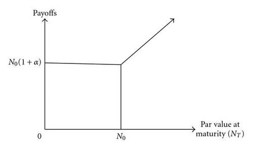
Index-linked and principal-protected notes are one of structured products. They have some properties. We can take an example to describe them. Assume that the initial (notional) par value of the notes is N0 per unit. Issuers promise at expiration (T) to deliver capital gains (NT − N0) and (1 + λ) portions of the initial par value if the par value at maturity NT is no fewer than N0, where λ is a constant guaranteed rate. Otherwise, issuers only pay (1 + λ) portions of the initial par value if the par value at maturity is less than the initial par value.
3. Model Checking
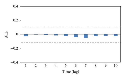
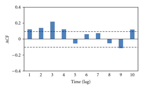
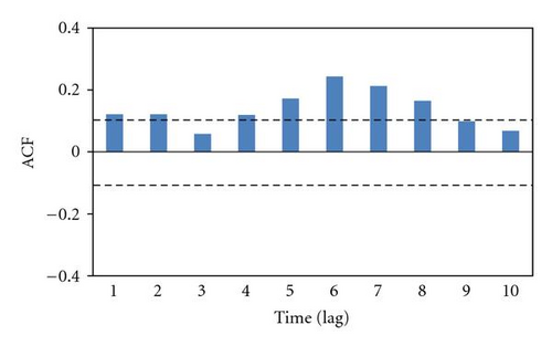
Consider the RUD, DJQ, and SPO notes, which are index-linked and principal-protected notes issued by Structures Products Corporation in USA. They are linked to Russel 2000 index, Dow Jones Industrial Average index, and S&P500, respectively. The samples in this study span from May 13, 2004, through April 30, 2008, or 997 daily log returns. Furthermore, WTI oil price is used to breakdown all of the samples into the low oil price years from May 13, 2004, to August 29, 2005, the high oil price years from August 30, 2005, to April 30, 2008, and the whole period from May 13, 2004, to April 30, 2008, because the time break occurred on August 30, 2005.
-
1 AR(1)-ARCH(p):
-
2 AR(1)-GARCH(p, q):
| Notes | Mean | Standard deviation | Skewness | Kurtosis | Q1 | Q2 |
|---|---|---|---|---|---|---|
| Panel A: May 13, 2004 to August 29, 2005 | ||||||
| RUD | −0.000228 | 0.008842 | −0.178742 | 2.808400 | 102.61 (0.128) | 26.59 (0.10) * |
| SPO | 0.000199 | 0.006508 | −0.278440 | 1.933470 | 71.63 (0.502) | 96.86 (0.00) * |
| DJQ | 0.000112 | 0.006409 | 0.299268 | 2.264748 | 59.54 (0.146) | 14.22 (0.00) * |
| Panel B: August 30, 2005 to April 30, 2008 | ||||||
| RUD | 0.000168 | 0.007301 | −0.131015 | 3.071701 | 103.00 (0.116) | 35.25 (0.00) * |
| SPO | 0.000141 | 0.008853 | −0.295478 | 5.591546 | 71.63 (0.602) | 130.22 (0.00) * |
| DJQ | 0.000267 | 0.008166 | 0.117100 | 3.481814 | 61.75 (0.667) | 38.43 (0.00) * |
| Panel C: May 13, 2004 to April 30, 2008 | ||||||
| RUD | 0.000038 | 0.007838 | −0.168216 | 3.622114 | 91.6 (0.556) | 56.37 (0.00) * |
| SPO | 0.000160 | 0.008155 | −0.210099 | 5.647948 | 65.09 (0.117) | 159.87 (0.00) * |
| DJQ | 0.000216 | 0.007631 | 0.044427 | 3.550943 | 48.80 (0.667) | 58.72 (0.00) * |
- Note that mean, standard deviation, skewness, and kurtosis are for log returns. Q1 and Q2 stand for Ljung-Box statistics for log returns and squared log returns, respectively. P-values are in parentheses. The symbol *denotes significance at 10 percent level.


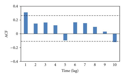
-
3 AR(1)-EGARCH(p, q):
In the above models, rt denotes the daily log returns at time t, εt stands for the shock at time t, and μ0, μ1, αi, βi, and γ represent constant coefficients.
Then, the order of these models is determined by means of AIC and SBIC. AIC and SBIC denote Akaike information criterion and Schwartz Bayesian information criterion, respectively. As stated in Table 2, AR(1)-ARCH(5), AR(1)-GARCH(1,1), AR(1)-GARCH(1,4), and AR(1)-EGARCH(1,1) are adequate for RUD because their AIC or SBIC is the smallest. Similarly, AR(1)-ARCH(5), AR(1)-GARCH(1,1), AR(1)-GARCH(2,5), and AR(1)-EGARCH(1,1) are suitable for SPO; AR(1)-ARCH(5), AR(1)-GARCH(2,1), AR(1)-GARCH(2,5), AR(1)-EGARCH(2,1), and AR(1)-EGARCH(2,2) are suitable for DJQ.
| Products | ||||||
|---|---|---|---|---|---|---|
| RUD notes | SPO notes | DJQ notes | ||||
| Time series models | AIC | SBIC | AIC | SBIC | AIC | SBIC |
| Panel A: AR(1)-ARCH(p) models | ||||||
| AR(1)-ARCH(1) | −6.941219 | −6.916461 | −6.959115 | −6.964556 | −6.985434 | −6.990375 |
| AR(1)-ARCH(2) | −6.958195 | −6.938517 | −6.978548 | −6.978360 | −6.999533 | −6.999365 |
| AR(1)-ARCH(3) | −6.956246 | −6.961649 | −6.987542 | −6.985925 | −7.214846 | −7.019248 |
| AR(1)-ARCH(4) | −6.959551 | −6.990034 | −6.999757 | −6.995240 | −7.335362 | −7.211805 |
| AR(1)-ARCH(5) | −6.969473 | −7.321037 | −7.204025 | −7.169589 | −7.443874 | −7.319038 |
| Panel B: AR(1)-GARCH(p, q) models | ||||||
| AR(1)-GARCH(1,1) | −7.061470 | −7.168470 | −7.134326 | −7.119648 | −7.198410 | −7.179732 |
| AR(1)-GARCH(1,2) | −7.061591 | −7.138694 | −7.133050 | −7.109452 | −7.189593 | −7.178995 |
| AR(1)-GARCH(1,3) | −7.067123 | −7.137606 | −7.140847 | −7.111330 | −7.171505 | −7.177988 |
| AR(1)-GARCH(1,4) | −7.079660 | −7.138223 | −7.139879 | −7.105443 | −7.154642 | −7.066206 |
| AR(1)-GARCH(1,5) | −7.078558 | −7.133202 | −7.138095 | −7.108739 | −7.128017 | −7.055761 |
| AR(1)-GARCH(2,1) | −7.069515 | −7.141917 | −7.134357 | −7.107760 | −7.101990 | −7.179393 |
| AR(1)-GARCH(2,2) | −7.066915 | −7.139598 | −7.130790 | −7.103273 | −7.100254 | −7.170737 |
| AR(1)-GARCH(2,3) | −7.067199 | −7.132742 | −7.141224 | −7.105788 | −7.193758 | −7.165321 |
| AR(1)-GARCH(2,4) | −7.064881 | −7.124625 | −7.139171 | −7.108815 | −7.197960 | −7.158604 |
| AR(1)-GARCH(2,5) | −7.062167 | −7.122891 | 7.145930 | −7.108954 | −7.209054 | −7.144778 |
| Panel C: AR(1)-EGARCH(p, q) models | ||||||
| AR(1)-EGARCH(1,1) | −7.179744 | −7.156460 | −7.179744 | −7.155146 | −7.192009 | −7.167411 |
| AR(1)-EGARCH(1,2) | −7.178005 | −7.148488 | −7.178005 | −7.148488 | −7.197912 | −7.168395 |
| AR(1)-EGARCH(1,3) | −7.176422 | −7.141386 | −7.176422 | −7.141986 | −7.199830 | −7.165393 |
| AR(1)-EGARCH(1,4) | −7.177734 | −7.140878 | −7.179734 | −7.140378 | −7.197992 | −7.158636 |
| AR(1)-EGARCH(1,5) | −7.178635 | −7.139360 | −7.179635 | −7.135360 | −7.196798 | −7.152522 |
| AR(1)-EGARCH(2,1) | −7.177352 | −7.098235 | −7.177752 | −7.148235 | −7.199603 | − 7.170086 |
| AR(1)-EGARCH(2,2) | −7.176270 | −7.091833 | −7.176270 | −7.141833 | −7.203197 | −7.168760 |
| AR(1)-EGARCH(2,3) | −7.175279 | −7.089923 | −7.178279 | −7.139923 | −7.208211 | −7.158855 |
| AR(1)-EGARCH(2,4) | −7.165957 | − 7.094681 | −7.178957 | −7.134681 | −7.207023 | −7.152748 |
| AR(1)-EGARCH(2,5) | −7.165842 | −7.098747 | −7.177942 | −7.128747 | −7.207152 | −7.150856 |
- Note that AIC and SBIC denote Akaike information criterion and Schwartz Bayesian information criterion, respectively.
The estimation of the selected models is shown in Table 3 during the three periods—the whole period, the low oil price period, and the high oil price period. In next section, the results of the estimation of these selected models are used to measure VaRs of index-linked and principal-protected notes.
| RUD notes | ||||||||||
|---|---|---|---|---|---|---|---|---|---|---|
| Time series models | Parameter | |||||||||
| Panel A: The whole period | ||||||||||
| μ | α0 | α1 | α2 | α3 | α4 | α5 | RMSE | MAE | ||
| AR(1)-ARCH(5) | 0.000075 | 0.000133 | 0.224618 | 0.155303 | −0.123168 | 0.091281 | 0.070586 | 0.007834 | 0.005241 | |
| μ | α0 | α1 | β1 | |||||||
| AR(1)-GARCH(1,1) | 0.001243 | 0.000123 | 0.141169 | 0.814768 | 0.007834 | 0.005246 | ||||
| μ | α0 | α1 | β1 | β2 | β3 | β4 | ||||
| AR(1)-GARCH(1,4) | 0.001139 | 0.000134 | 0.152539 | 0.664518 | −0.343514 | 0.887827 | −0.41614 | 0.007834 | 0.005236 | |
| μ | α0 | α1 | γ | β1 | ||||||
| AR(1)-EGARCH(1,1) | 0.001513 | -1.465525 | 0.432311 | 0.211102 | 0.7875371 | 0.007848 | 0.005224 | |||
| Panel B: The low oil price period | ||||||||||
| μ | α0 | α1 | α2 | α3 | α4 | α5 | RMSE | MAE | ||
| AR(1)-ARCH(5) | −0.001177 | 0.001250 | 0.123340 | 0.087360 | −0.033873 | 0.123157 | 0.062676 | 0.007835 | 0.005246 | |
| μ | α0 | α1 | β1 | |||||||
| AR(1)-GARCH(1,1) | −0.001377 | 0.000118 | 0.112652 | 0.811888 | 0.007840 | 0.005291 | ||||
| μ | α0 | α1 | β1 | β2 | β3 | β4 | ||||
| AR(1)-GARCH(1,4) | −0.0002145 | 0.000113 | 0.166107 | 0.566635 | −0.416205 | 0.718833 | −0.344506 | 0.007837 | 0.005272 | |
| μ | α0 | α1 | γ | β1 | ||||||
| AR(1)-EGARCH(1,1) | 0.001235 | −10.5564833 | 0.223816 | 0.212933 | −0.088939 | 0.007302 | 0.005282 | |||
| Panel C: The high oil price period | ||||||||||
| μ | α0 | α1 | α2 | α3 | α4 | α5 | RMSE | MAE | ||
| AR(1)-ARCH(5) | 0.001123 | 0.001137 | 0.245690 | 0.237896 | −0.013347 | −0.035673 | 0.071133 | 0.007295 | 0.004973 | |
| μ | α0 | α1 | β1 | |||||||
| AR(1)-GARCH(1,1) | 0.000334 | 0.000102 | 0.177786 | 0.799431 | 0.007294 | 0.004967 | ||||
| μ | α0 | α1 | β1 | β2 | β3 | β4 | ||||
| AR(1)-GARCH(1,4) | 0.001132 | 0.000103 | 0.245556 | 0.789879 | −0.539841 | 0.245112 | 0.217447 | 0.007294 | 0.004968 | |
| μ | α0 | α1 | γ | β1 | ||||||
| AR(1)-EGARCH(1,1) | 0.000551 | −1.126772 | 0.343221 | 0.132112 | 0.912626 | 0.007302 | 0.005011 | |||
| SPO notes | ||||||||||
| Time series models | Parameter | |||||||||
| Panel A: The whole period | ||||||||||
| μ | α0 | α1 | α2 | α3 | α4 | α5 | RMSE | MAE | ||
| AR(1)-ARCH(5) | 0.000778 | 0.000102 | 0.124557 | 0.166728 | 0.098039 | 0.234964 | 0.567833 | 0.008156 | 0.005566 | |
| μ | α0 | α1 | β1 | |||||||
| AR(1)-GARCH(1,1) | 0.000665 | 0.000112 | 0.099794 | 0.991196 | 0.008553 | 0.005556 | ||||
| μ | α0 | α1 | α2 | β1 | β2 | β3 | β4 | β5 | ||
| AR(1)-GARCH(2,5) | 0.001520 | 0.000112 | 0.088600 | 0.075643 | 0.823604 | −0.4127508 | 0.665673 | −0.888641 | 0.882347 | |
| 0.008155 | 0.005565 | |||||||||
| μ | α0 | α1 | γ | β1 | ||||||
| AR(1)-EGARCH(1,1) | 0.000558 | −0.366564 | 0.213535 | 0.005563 | 0.988207 | 0.008157 | 0.005570 | |||
| Panel B: The low oil price period | ||||||||||
| μ | α0 | α1 | α2 | α3 | α4 | α5 | RMSE | MAE | ||
| AR(1)-ARCH(5) | 0.000112 | 0.000138 | 0.096679 | −0.002138 | −0.041125 | 0.089648 | 0.134568 | 0.008152 | 0.005520 | |
| μ | α0 | α1 | β1 | |||||||
| AR(1)-GARCH(1,1) | 0.000114 | 0.000211 | 0.048385 | 0.933170 | 0.008152 | 0.005547 | ||||
| μ | α0 | α1 | α2 | β1 | β2 | β3 | β4 | β5 | ||
| AR(1)-GARCH(2,5) | 0.000719 | 0.0001122 | 0.111361 | −0.088981 | 0.397539 | 0.0311331 | 0.385764 | 0.299079 | −0.21435 | |
| 0.008152 | 0.005525 | |||||||||
| μ | α0 | α1 | γ | β1 | ||||||
| AR(1)-EGARCH(1,1) | 0.001122 | −5.998389 | 0.064714 | 0.299825 | 0.455299 | 0.008163 | 0.005585 | |||
| Panel C: The high oil price period | ||||||||||
| μ | α0 | α1 | α2 | α3 | α4 | α5 | RMSE | MAE | ||
| AR(1)-ARCH(5) | 0.000565 | 0.000078 | 0.114599 | 0.211361 | 0.121363 | 0.097749 | 0.056788 | 0.008874 | 0.005949 | |
| μ | α0 | α1 | β1 | |||||||
| AR(1)-GARCH(1,1) | 0.000394 | 0.000113 | 0.126451 | 0.866762 | 0.008874 | 0.005949 | ||||
| μ | α0 | α1 | α2 | β1 | β2 | β3 | β4 | β5 | ||
| AR(1)-GARCH(2,5) | 0.001233 | 0.0001124 | 0.126651 | 0.088795 | 0.611582 | -0.113913 | 0.311316 | −0.711249 | 0.698910 | |
| 0.008874 | 0.005949 | |||||||||
| μ | α0 | α1 | γ | β1 | ||||||
| AR(1)-EGARCH(1,1) | 0.000778 | −0.512671 | 0.256784 | 0.044575 | 0.958854 | 0.008884 | 0.005969 | |||
| DJQ notes | ||||||||||
| Time series models | Parameter | |||||||||
| Panel A: The whole period | ||||||||||
| μ | α0 | α1 | α2 | α3 | α4 | α5 | RMSE | MAE | ||
| AR(1)-ARCH(5) | 0.000443 | 0.000113 | 0.211583 | 0.13348 | 0.114672 | 0.11126 | 0.066886 | 0.007630 | 0.005398 | |
| μ | α0 | α1 | α2 | β1 | ||||||
| AR(1)-GARCH(2,1) | 0.001130 | 0.000121 | 0.215542 | -0.131214 | 0.889394 | 0.007628 | 0.005391 | |||
| μ | α0 | α1 | α2 | β1 | β2 | β3 | β4 | β5 | ||
| AR(1)-GARCH(2,5) | 0.001137 | 0.000111 | 0.188956 | -0.177846 | 1.184288 | 0.418862 | -0.340559 | -0.811254 | 0.526681 | |
| 0.007629 | 0.005395 | |||||||||
| μ | α0 | α1 | α2 | γ | β1 | |||||
| AR(1)-EGARCH(2,1) | 0.000313 | -0.281558 | 0.378891 | -0.221350 | -0.011877 | 0.898797 | 0.007628 | 0.005389 | ||
| μ | α0 | α1 | α2 | γ | β1 | β2 | ||||
| AR(1)-EGARCH(2,2) | 0.001134 | -0.055808 | 0.411404 | -0.311069 | -0.021166 | 1.566290 | -0.778983 | 0.007628 | 0.005392 | |
| Panel B: The low oil price period | ||||||||||
| μ | α0 | α1 | α2 | α3 | α4 | α5 | RMSE | MAE | ||
| AR(1)-ARCH(5) | -0.000113 | 0.000167 | 0.322399 | 0.099110 | 0.026004 | -0.021233 | -0.045188 | 0.007632 | 0.005377 | |
| μ | α0 | α1 | α2 | β1 | ||||||
| AR(1)-GARCH(2,1) | 0.0001083 | 0.000112 | 0.466754 | -0.055689 | 0.244596 | 0.007631 | 0.003701 | |||
| μ | α0 | α1 | α2 | β1 | β2 | β3 | β4 | β5 | ||
| AR(1)-GARCH(2,5) | -0.000116 | 0.000111 | 0.356711 | -0.211299 | 0.611261 | 0.088741 | -0.091258 | 0.021123 | -0.092397 | |
| 0.007633 | 0.005382 | |||||||||
| μ | α0 | α1 | α2 | γ | β1 | |||||
| AR(1)-EGARCH(2,1) | 0.000441 | -5.522416 | 0.622357 | -0.055101 | 0.211319 | 0.511383 | 0.007628 | 0.005390 | ||
| μ | α0 | α1 | α2 | γ | β1 | β2 | ||||
| AR(1)-EGARCH(2,2) | 0.000668 | -13.512605 | 0.694437 | 0.711222 | 0.112577 | - 0.391220 | 0.181336 | 0.007628 | 0.005386 | |
| Panel C: The high oil price period | ||||||||||
| μ | α0 | α1 | α2 | α3 | α4 | α5 | RMSE | MAE | ||
| AR(1)-ARCH(5) | 0.000771 | 0.000123 | 0.144517 | 0.133165 | 0.171292 | 0.213814 | 0.113118 | 0.008166 | 0.005746 | |
| μ | α0 | α1 | α2 | β1 | ||||||
| AR(1)-GARCH(2,1) | 0.001124 | 0.000111 | 0.161129 | -0.033211 | 0.877278 | 0.008160 | 0.005744 | |||
| μ | α0 | α1 | α2 | β1 | β2 | β3 | β4 | β5 | ||
| AR(1)-GARCH(2,5) | 0.001125 | 0.000111 | 0.111213 | -0.088396 | 1.112524 | 0.733184 | -0.491514 | -0.988785 | 0.772727 | |
| 0.008160 | 0.0057435 | |||||||||
| μ | α0 | α1 | α2 | γ | β1 | |||||
| AR(1)-EGARCH(2,1) | 0.001145 | -0.413491 | 0.222399 | -0.011715 | -0.001136 | 0.982226 | 0.008160 | 0.005744 | ||
| μ | α0 | α1 | α2 | γ | β1 | β2 | ||||
| AR(1)-EGARCH(2,2) | 0.000661 | -0.534123 | 0.277669 | 0.099854 | 0.015515 | 0.0414396 | 0.581893 | 0.008161 | 0.005744 | |
- Note that RMSE and MAE demonstrate root mean squared errors and mean absolute errors, respectively.
4. Accuracy Evaluation
This section will conduct accuracy evaluation of selected time series models for VaR forecast by backtesting method, the multivariate extension of Diebold and Mariano test, RMSE, and MAE. Before backtesting method, it is necessary to calculate VaRs for these three kinds of securities.
4.1. VaR Measurement and Implication
| Time series model | The whole period | The low oil period | The high oil period | ||||||
|---|---|---|---|---|---|---|---|---|---|
| E(rt(1)) | VaR | E(rt(1)) | VaR | E(rt(1)) | VaR | ||||
| Panel A: RUD notes | |||||||||
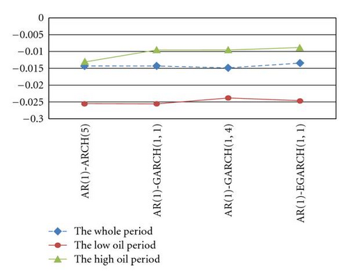
| AR(1)-ARCH(5) | 0.000084 | 0.000052 | −0.014279 | 0.000088 | 0.000121 | −0.025542 | 0.000283 | 0.000033 | −0.013179 |
| AR(1)-GARCH(1,1) | 0.000101 | 0.000038 | −0.014262 | 0.000265 | 0.000124 | −0.025681 | 0.000247 | 0.000017 | −0.009498 |
| AR(1)-GARCH(1,4) | 0.000041 | 0.000041 | −0.014878 | 0.000212 | 0.000106 | −0.023770 | 0.000252 | 0.000018 | −0.009531 |
| AR(1)-EGARCH(1,1) | 0.000512 | 0.000036 | −0.013468 | 0.000312 | 0.000115 | −0.024674 | 0.000502 | 0.000016 | −0.008866 |
| Panel B: SPO notes | |||||||||
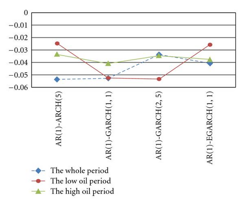
| AR(1)-ARCH(5) | 0.000512 | 0.000541 | −0.053682 | 0.000112 | 0.000112 | −0.024546 | 0.000412 | 0.000211 | −0.033433 |
| AR(1)-GARCH(1,1) | 0.000426 | 0.000521 | −0.052757 | 0.000312 | 0.000512 | −0.052410 | 0.000408 | 0.000312 | −0.040748 |
| AR(1)-GARCH(2,5) | 0.000451 | 0.000212 | −0.033474 | 0.000122 | 0.000552 | −0.053312 | 0.000410 | 0.000224 | −0.034462 |
| AR(1)-EGARCH(1,1) | 0.000554 | 0.000312 | −0.040602 | 0.000613 | 0.000126 | −0.025541 | 0.000511 | 0.000266 | −0.037490 |
| Panel C: DJQ notes | |||||||||
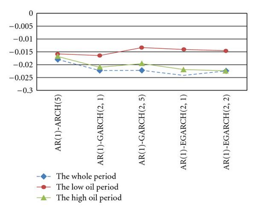
| AR(1)-ARCH(5) | 0.000405 | 0.000062 | −0.017941 | 0.000056 | 0.000460 | −0.015747 | 0.000671 | 0.000056 | −0.016745 |
| AR(1)-GARCH(2,1) | 0.000311 | 0.000094 | −0.022279 | 0.000013 | 0.000049 | −0.016297 | 0.000524 | 0.000085 | −0.020957 |
| AR(1)-GARCH(2,5) | 0.000377 | 0.000093 | −0.022093 | 0.000086 | 0.000033 | −0.013299 | 0.000495 | 0.000074 | −0.019496 |
| AR(1)-EGARCH(2,1) | 0.000293 | 0.000110 | −0.024144 | 0.000366 | 0.000038 | −0.013997 | 0.000505 | 0.000092 | −0.021838 |
| AR(1)-EGARCH(2,2) | 0.000364 | 0.000095 | −0.022346 | 0.000258 | 0.000040 | −0.014478 | 0.000536 | 0.000096 | −0.022247 |
- Note that the VaRs are for a one-day-ahead horizon and a 99% confidence level for losses. E[rt(1)] and denote the expected value and the forecast variance of asset returns over a one-period horizon, respectively.
Table 4 indicates that the VaRs based on GARCH-type models are the smallest for RUD notes in the whole period and low oil price period; the VaRs in AR(1)-ARCH(5) model are the smallest in high oil price period. This implies that in the GARCH-type models, it is necessary for financial investors to keep the greatest need of a minimum solvency safety margin because the worst potential losses of the models are the largest than the other models in the whole period and low oil price period. Meanwhile, the result is low profitability of the return on equity (ROE) and downward pressure on the bank’s stock price during the whole and low oil price periods. Similarly, the phenomena occur in the AR(1)-ARCH(5) model in the high oil price period.
As for SPO notes, the minimum VaRs happen in the GARCH-type models during the low and high oil price periods; the VaR of the AR(1)-ARCH(5) model is the lowest among those of the other models in the whole period. Hence, it is necessary for a bank to maintain the maximum capital amount in order to prevent from default risk in terms of the GARCH-type models during the low oil price and high oil price periods. However, the need of a minimum solvency safety margin under the AR(1)-ARCH(5) model is the greatest during the whole period.
Again, for DJQ notes, the VaRs measured by the EGARCH-type models are the smallest in the whole and high oil price periods; the capital requirement of the AR(1)-GARCH(2,1) model is the largest in the low oil price period.
To sum up, there exists a consistent phenomenon that the VaRs of GARCH-type models are the smallest among those of the selected models during the low oil price period. When financial risk managers employ GARCH-type models to measure VaRs during the low oil price period, the firm’s default risk can fall because of sufficient capital requirement. In general, the worst potential losses of ARCH-type models are fewer than those of GARCH-type models during the three periods. On account of the increase of costs during the high oil price period, it would be better for banks to use ARCH-type models to manage market risk in order not to worsen the profitability.
On the other hand, there is also an interesting phenomenon that the amounts of VaRs are independent of economic situations as illustrated in Figure 4. That is different from common sense that the worse the economic situation is, the larger VaRs are to prevent from bankruptcy.
4.2. Backtesting Method
As shown in Table 5, Panel A illustrates that the null hypothesis is rejected in AR(1)-ARCH(5), AR(1)-GARCH(1,1), AR(1)-GARCH(1,4), and AR(1)-EGARCH(1,1) models for RUD notes in the whole and the high oil price periods. It implies that these models are not suitable for a 1% significance level in the whole period and the high oil price period while 1% is the true probability for AR(1)-ARCH(5) and AR(1)-GARCH(1,1) in the low oil price period. Again, as stated in Panel B, one fails to reject the null hypothesis in AR(1)-GARCH(2,5) and AR(1)-ARCH(5) models for SPO notes in the whole period and in the low oil price period, respectively, whereas both AR(1)-GARCH(2,5) and AR(1)-ARCH(5) models are fit for a 1% significance level during the high oil price period. As for DJQ notes illustrated in Panel C, all of selected models are not fit for a 1% significance level in the low oil price period. However, one accepts the null hypothesis for AR(1)-GARCH(2,1) and EGARCH-type models in the whole period and the high oil price period.
| Time series model | The whole period | The low oil period | The high oil period | ||||||
|---|---|---|---|---|---|---|---|---|---|
| Total number | Exception | LR | Total number | Exception | LR | Total number | Exception | LR | |
| Panel A: RUD notes | |||||||||
| AR(1)-ARCH(5) | 997 | 44 | 63.7726 * | 326 | 5 | 0.8065 | 671 | 29 | 41.0709 * |
| AR(1)-GARCH(1,1) | 997 | 72 | 164.6229 * | 326 | 5 | 0.8065 | 671 | 56 | 142.8076 * |
| AR(1)-GARCH(1,4) | 997 | 64 | 132.9438 * | 326 | 14 | 19.6867 * | 671 | 56 | 142.8076 * |
| AR(1)-EGARCH(1,1) | 997 | 79 | 193.9234 * | 326 | 11 | 11.4628 * | 671 | 64 | 179.1857* |
| Panel B: SPO notes | |||||||||
| AR(1)-ARCH(5) | 997 | 1 | 13.42211 * | 326 | 2 | 0.5706 | 671 | 5 | 0.4828 |
| AR(1)-GARCH(1,1) | 997 | 1 | 13.42211 * | 326 | 0 | 6.5528 * | 671 | 1 | 7.6617 * |
| AR(1)-GARCH(2,5) | 997 | 5 | 3.0636 | 326 | 0 | 6.5528 * | 671 | 7 | 0.0125 |
| AR(1)-EGARCH(1,1) | 997 | 2 | 9.5784 * | 326 | 0 | 6.5528 * | 671 | 2 | 4.6115* |
| Panel C: DJQ notes | |||||||||
| AR(1)-ARCH(5) | 997 | 27 | 20.0334 * | 326 | 13 | 16.7807 * | 671 | 20 | 17.3730 * |
| AR(1)-GARCH(2,1) | 997 | 10 | 0.0001 | 326 | 13 | 16.7807 * | 671 | 11 | 2.3223 |
| AR(1)-GARCH(2,5) | 997 | 12 | 0.3920 | 326 | 17 | 29.2640 * | 671 | 13 | 4.6749 * |
| AR(1)-EGARCH(2,1) | 997 | 12 | 0.3920 | 326 | 14 | 19.6867 * | 671 | 8 | 0.2360 |
| AR(1)-EGARCH(2,2) | 997 | 9 | 0.0985 | 326 | 11 | 11.4628 * | 671 | 8 | 0.2360 |
- Note that the symbol *denotes a 5% critical value of 3.84. LR demonstrates an unconditional coverage.
4.3. Multivariate Extension of Diebold and Mariano Test
Following the suggestions of past studies that GARCH model tends to have better performance in evaluating volatility, this paper uses the GARCH model to be a benchmark to compete with the other time series models selected. It is worthwhile noticing that the square errors of volatility are the gap between actual volatility (measured by a squared daily return) and the volatility generated by models.
As shown in Table 6, Panel A demonstrates that there is no significant difference in the accuracy of the couple competing models for RUD notes during the whole period when the benchmark is based on the GARCH-type models. The constant coefficient are not significantly positive in AR(1)-ARCH(5) and not significantly negative in AR(1)-GARCH(1,4) and AR(1)-EGARCH(1,1). It implies that the performances of AR(1)-GARCH(1,1) are not significantly worse than those of AR(1)-ARCH(5), while not significantly better than those of AR(1)-EGARCH(1,1) and AR(1)-GARCH(1,4). Alternatively, based on AR(1)-GARCH(1,4) as a benchmark, AR(1)-GARCH(1,4) is not significantly worse than the other selected models for RUD notes in the whole period. Therefore, as for RUD notes, there is no forecasting model that consistently has a superior performance in the whole period. Following the vein, the GARCH-type models do not significantly perform a better accuracy than AR(1)-ARCH(5) and AR(1)-EGARCH(1,1) in the low oil price period; their performance is not significantly better than that of AR(1)-ARCH(5) model but not significantly worse than that of AR(1)-EGARCH(1,1) in the high oil price period.
| RUD notes | SPO notes | DJQ notes | ||||||
|---|---|---|---|---|---|---|---|---|
| Explained variables | Constant | P-value | Explained variables | Constant | P-value | Explained variables | Constant | P-value |
| Panel A: The whole period | ||||||||
| Based on AR(1)-GARCH(1,1) | Based on AR(1)-GARCH(1,1) | Based on AR(1)-GARCH(2,1) | ||||||
| Y1 | 0.001522 | .9985 | Z1 | 0.002467 | .9445 | W1 | −0.002134 | .9779 |
| Y2 | −0.001387 | .9828 | Z2 | −0.003968 | .9806 | W2 | −0.054672 | .6081 |
| Y3 | −0.002345 | .9988 | Z3 | 0.004578 | .9562 | W3 | −0.009875 | .9198 |
| W4 | −0.001236 | .6804 | ||||||
| Based on AR(1)- GARCH(1,4) | Based on AR(1)- GARCH(2,5) | Based on AR(1)-GARCH(2,5) | ||||||
| Y1 | 0.004587 | .9865 | Z1 | 0.001346 | .9393 | W1 | 0.007895 | .8057 |
| Y2 | 0.007895 | .9828 | Z2 | 0.008795 | .9806 | W2 | 0.008875 | .6080 |
| Y3 | 0.003547 | .9972 | Z3 | 0.006458 | .9606 | W3 | 0.001246 | .6638 |
| W4 | 0.003746 | .8244 | ||||||
| Panel B: The low oil price period | ||||||||
| Based on AR(1)-GARCH(1,1) | Based on AR(1)-GARCH(1,1) | Based on AR(1)-GARCH(2,1) | ||||||
| Y1 | −0.011483 | .4723 | Z1 | −0.036871 | .4544 | W1 | −0.002246 | .9776 |
| Y2 | −0.022464 | .9824 | Z2 | −0.054692 | .3373 | W2 | −0.007854 | .6629 |
| Y3 | −0.044785 | .9555 | Z3 | 0.001458 | .8565 | W3 | 0.001365 | .9462 |
| W4 | 0.004789 | .9498 | ||||||
| Based on AR(1)-GARCH(1,4) | Based on AR(1)-GARCH(2,5) | Based on AR(1)-GARCH(2,5) | ||||||
| Y1 | −0.001456 | .6626 | Z1 | −0.001648 | .8451 | W1 | 0.006591 | .9162 |
| Y2 | 0.008964 | .9824 | Z2 | 0.001935 | .4916 | W2 | 0.003169 | .6629 |
| Y3 | −0.003659 | .9745 | Z3 | 0.008934 | .4916 | W3 | 0.007598 | .7091 |
| W4 | 0.001564 | .7206 | ||||||
| Panel C: The high oil price period | ||||||||
| Based on AR(1)-GARCH(1,1) | Based on AR(1)-GARCH(1,1) | Based on AR(1)-GARCH(2,1) | ||||||
| Y1 | −0.004136 | .7441 | Z1 | −0.002156 | .8925 | W1 | −0.006647 | .1296 |
| Y2 | −0.002159 | .9668 | Z2 | 0.001489 | .9104 | W2 | −0.009917 | .0219* |
| Y3 | 0.007845 | .9871 | Z3 | −0.007156 | .9825 | W3 | 0.007814 | .9757 |
| W4 | −0.001398 | .9188 | ||||||
| Based on AR(1)-GARCH(1,4) | Based on AR(1)- GARCH(2,5) | Based on AR(1)-GARCH(2,5) | ||||||
| Y1 | −0.009551 | .7531 | Z1 | −0.002346 | .8344 | W1 | 0.001754 | .1854 |
| Y2 | 0.007415 | .9668 | Z2 | −0.002805 | .9104 | W2 | 0.004879 | .0219* |
| Y3 | 0.001365 | .9656 | Z3 | −0.003224 | .9099 | W3 | 0.003456 | .2122 |
| W4 | 0.003099 | .2978 | ||||||
- Note that Y1 and Y3 stand for the differences of the sum of squared errors (SSEs) of volatility in GARCH from AR(1)-ARCH(5) and AR(1)-EGARCH(1,1), respectively. Y2 denotes the differences of SSE of volatility in AR(1)-GARCH(1,1) from AR(1)-GARCH(1,4) as the benchmark is AR(1)-GARCH(1,1). Conversely, when the benchmark is AR(1)-GARCH(1,4),Y2 represents the differences of SSE of volatility in AR(1)-GARCH(1,4) from AR(1)-GARCH(1,1). Z1 and Z3 stand for the differences of SSE of volatility in AR(1)-GARCH from AR(1)-ARCH(5) and AR(1)-EGARCH(1,1), respectively. Z2 denotes the differences of SSE of volatility in AR(1)-GARCH(1,1) from GARCH(2,5) as the benchmark is GARCH(1,1). Conversely, when the benchmark is GARCH(2,5), Y2 represents the differences of SSE of volatility in AR(1)-GARCH(2,5) from AR(1)-GARCH(1,1).W1, W3, and W4 stand for the differences of the sum of SSE of volatility in AR(1)-GARCH from AR(1)-ARCH(5), AR(1)-EGARCH(2,1), and AR(1)-EGARCH(2,2), respectively. W2 denotes the differences of SSE of volatility in AR(1)-GARCH(2,1) from AR(1)-GARCH(2,5) as the benchmark is AR(1)-GARCH(2,1). Conversely, when the benchmark is AR(1)-GARCH(2,5), Y2 represents the differences of SSE of volatility in AR(1)-GARCH(2,5) from AR(1)-GARCH(2,1).The symbol * denotes significance at 5 percent level.
As for SPO, the GARCH-type models are not significantly worse than the other models in the whole period; it is not significantly better than AR(1)-ARCH(5) but not significantly worse than AR(1)-EGARCH(1,1) in the low oil price period. GARCH-type models are not significantly better than both AR(1)-ARCH(5) and AR(1)-EGARCH(1,1) models during the high oil period. Hence the accuracy of AR(1)-ARCH(5) model is relatively better than the GARCH-type models during both low oil price and high oil price periods.
Similarly, as for DJQ, the accuracy performance for AR(1)-GARCH(2,1) model is not significantly higher than AR(1)-ARCH(5), AR(1)-EGARCH(2,1), and AR(1)-EGARCH(2,2) in both the whole and low oil periods. Contrary, AR(1)-ARCH(5), AR(1)-EGARCH(2,1), and AR(1)-EGARCH(2,2) models are not significantly better than AR(1)-GARCH(2,5) model in the high oil price period.
Return to Table 3. We apply RMSE and MAE to evaluate the accuracy of selected models. If the RMSE or MAE of a model is low, it stands for the accuracy of the model being better than the other.
As for RUD notes, one can find that the RMSEs (root mean squared errors) of AR(1)-ARCH(5), AR(1)-GARCH(1,1), and AR(1)-GARCH(1,4) and the MAE of AR(1)-EGARCH(1,1) are the smallest in the whole period; the RMSE of AR(1)-EGARCH(1,1) and the MAE of AR(1)-ARCH(5) are the lowest in the low oil price period; the RMSE and MAE of the GARCH-type models are the minimum in the high oil price period.
Also for SPO notes, the RMSE and MAE of the GARCH-type models are the smallest in the whole period, while the RMSE and MAE are the minimum in AR(1)-ARCH(5) model during the low oil price period. In the high oil price period, AR(1)-ARCH(5) and GARCH-type models have the lowest RMSE and MAE among the other selected models.
There is a common phenomenon for DJQ notes that the RMSE of EGARCH-type models is the lowest in any period. On the other hand, the accuracy of the GARCH-type models measured by MAE is better in both low oil price and high oil price periods.
Finally, we summarize the overall results in terms of backtesting method, the multivariate extension of Diebold and Mariano test, MAE, and MSE as illustrated in Table 7. There seems to be no forecasting model that consistently has superior performance based on these criteria. However, Table 7 reports that in spite of RUD, SPO, and DJQ notes, the frequency of the better performance for the GARCH-type models is higher than that of the ARCH model and the EGARCH-type models in the whole period, whereas it is not in the low price period and the high oil price periods. The accuracy of EGARCH models seems to be worse than that of the other models for the index-linked and principal-protected notes in the whole period, the low oil price period, and the high oil price period
| Time series model | Backtesting | Multivariate extension of Diebold and Mariano test | RMSE | MAE | ||||||||
|---|---|---|---|---|---|---|---|---|---|---|---|---|
| W | L | H | W | L | H | W | L | H | W | L | H | |
| Panel A: RUD notes | ||||||||||||
| AR(1)-ARCH(5) | NB | B | NB | NB | B | B | B | NB | NB | NB | B | NB |
| AR(1)-GARCH(1,1) | NB | B | NB | B | NB | NB | B | NB | B | NB | NB | B |
| AR(1)-GARCH(1,4) | NB | NB | NB | B | NB | NB | B | NB | B | NB | NB | B |
| AR(1)-EGARCH(1,1) | NB | NB | NB | NB | B | NB | NB | B | NB | B | NB | NB |
| Panel B: SPO notes | ||||||||||||
| AR(1)-ARCH(5) | NB | B | B | NB | B | NB | B | B | NB | NB | B | B |
| AR(1)-GARCH(1,1) | NB | NB | NB | B | NB | B | B | B | B | B | NB | B |
| AR(1)-GARCH(2,5) | B | NB | B | B | NB | B | B | B | B | B | NB | B |
| AR(1)-EGARCH(1,1) | NB | NB | NB | NB | NB | NB | NB | NB | NB | NB | NB | NB |
| Panel C: DJQ notes | ||||||||||||
| AR(1)-ARCH(5) | NB | NB | NB | NB | NB | B | NB | NB | NB | NB | NB | NB |
| AR(1)-GARCH(2,1) | B | NB | B | B | B | NB | B | NB | B | NB | B | B |
| AR(1)-GARCH(2,5) | B | NB | NB | B | B | NB | B | NB | B | NB | B | B |
| AR(1)-EGARCH(2,1) | B | NB | B | NB | NB | B | B | B | B | B | NB | NB |
| AR(1)-EGARCH(2,2) | B | NB | B | NB | NB | B | B | B | B | B | NB | NB |
- Note that W, L, and H stand for the whole period, the low oil price period, and the high oil price period, respectively. NB and B denote “not better” and “better”, respectively. RMSE and MAE demonstrate root mean squared errors and mean absolute errors, respectively.
5. Conclusion
Because VaR is a function of volatility, volatility forecast is the main issue of VaR. In this paper, using backtesting method, the multivariate extension of Diebold and Mariano test, RMSE, and MAE, we find that there seems to be no forecasting model that consistently has superior performance based on these criteria. But, the performance of the GARCH-type models is probably better than that of ARCH and EGARCH in the whole period, while it is not in the low price period and the high oil price periods. Despite in the low oil price and the high oil price period, ARCH model seems to have superior performance for stock index-linked and principal-protected notes.
Additionally, it is worthy of note for banks to manage market risk that the VaRs of GARCH-type and EGARCH-type models are generally smaller during these three periods. It also means that GARCH and EGARCH produce higher capital requirements with respect to ARCH model in order to avoid default risks. As a result, the profitability in the GARCH-type and EGARCH-type models is lower. Thus, GARCH-type and EGARCH-type models further dampen a bank’s financial statement during the high oil price period. We suggest that in a boom economy, GARCH-type and EGARCH-type models can be provided to manage market risk for financial institutions whereas ARCH model would be adequate to a recession economy.
Alternatively, we find that the amounts of VaRs are independent of economy scenarios as illustrated in Figure 4. That is different from common sense that the worse the economic situation is, the larger VaRs are to prevent from bankruptcy.


