We present a remote, differential method for measuring the prescription of aspheric mirrors using null interferometry in the center-of-curvature configuration. The method requires no equipment beyond that used in a basic interferometery setup (i.e., there are no shearing elements or absolute distance meters). We chose this configuration because of its widespread use. However, the method is generalizable to other configurations with an adjustment of the governing equation. The method involves taking a series of interferograms before and after small, known misalignments are applied to the mirror in the interferometry setup and calculating the prescription (e.g., radius of curvature and conic constant) of the mirror, based on these differential measurements, using a nonlinear regression. We apply this method successfully to the testing of a Space Optics Research Lab off-axis parabola with a known focal length of 152.4 mm, a diameter of 76.2 mm, and an off-axis angle of 12°.

1. Introduction

An important problem in the realm of optical testing concerns the ability to remotely measure radius of curvature and conic constant of large reflective optical surfaces. Primary mirrors destined for space applications require cryogenic testing on the ground, during which their radii of curvature and conic constant can vary significantly and must be monitored. In such situations, the metrology instruments are located in a separate environment from the test mirror behind an optical window. Such remote measurements should be achievable with little or no equipment auxiliary to that normally used in interferometric figure testing. The radius of curvature and conic constant of large aperture optical surfaces in spaceborne instruments must also be monitored. In this situation as well, there is often a need to conduct an nonintrusive test of these shape parameters.

Methods currently exist for measuring the shapes of three-dimensional diffuse and specular objects in general [1] and of optical mirrors in particular [2]. But none of these methods answers the need for a simple, full-aperture, remote measurement technique that requires little more than the setup already used to do basic figure testing. Our approach is a differential method that involves deliberately misaligning the mirror in known magnitude and direction, measuring the effect via the interferogram, and regressing the parameters (e.g., conic constant and radius of curvature) that determine the mirror prescription, based on these effects. It is very important for the reader to note that, since this is a differential method, it is insensitive to residual misalignment and figure errors in the null optics, since they are subtracted out in the difference measurement. This paper begins in Section 2 by developing the theory based on the governing physical relationships. Then in Section 3, the nonlinear prescription regression is explained. Next in Section 4, the paper discusses experimental results obtained from testing an off-axis paraboloid using a null assembled from COTS optics, which introduces small but not insignificant wavefront errors, showing that the method works and is robust to null errors. Finally in Section 5, we conclude with a summary and a brief discussion of future directions.

2. Development of the Model Functions

In this section, building on earlier work by the authors [3], we first review the theory that explains the effects that misalignments have on the interferogram and how this depends on the mirror’s prescription. Then, based on this theory, we develop the linear model that will be used in each iteration of the the regression algorithm by making a first-order expansion. Next, we will consider the effects that errors in the orientation of the translation axes themselves have on our model. The axes along which we translate the mirror may not be coincident with the parent axes of the mirror itself and may be skewed with respect to each other. We will develop adjustments to the model which could be used to take this into account.

2.1. Misalignment-Induced Optical Path Difference (OPD)

A mathematical surface describing the mirror, with its explicit dependence on shape parameters, is written as the level surface

()

where z = f(x, y; θ₁, θ₂, …, θ_p) is the altitude function describing the two-dimensional surface, x and y are the pupil coordinates, and θ = (θ₁, θ₂, …, θ_p) is the vector of free shape parameters (e.g. radius of curvature and conic constant for the case of a conic surface). The unit surface normal is given in terms of the gradient of the level surface

()

and the optical path difference (OPD) δW caused by a rigid body displacement δr of the mirror is given by [3]

()

Equation (3) says that the OPD incurred at the point (x, y) due to a small displacement of the surface is equal to the component of the displacement that is normal to the surface at that point. Translations in x, y, and z are denoted by ε_x, ε_y, and ε_z, and rotations about the x, y, and z axes are denoted by the small angles ϕ_x, ϕ_y, and ϕ_z, respectively. In this limit, all the operations of translation and rotation are commutative, and the vector δr can be written

()

The measurements in our test consist of arrays of OPD values (i.e., interferograms from a phase-shifting inteferometer), one for each pixel of the interferometer detector. We will now perform a decomposition of δW, in which the parameters θ remain free. For mirrors with circular pupils, like the one we tested, a decomposition of the OPD function in terms of the orthonormal Zernike polynomials is convenient. Whatever the shape of the pupil, there will exist a complete orthonormal basis for functions defined on that pupil. One can derive such an orthonormal set via Gram-Schmidt procedures [4]. If we denote our set of orthonormal basis functions as {P_i(x, y)} and the set of coefficients in the expansion of the OPD function as {b_i}, we can expand (3) as

()

where the coefficients in the expansion, owing to their orthonormality, are given by

()

Using (3), (4), (5), and (6), we obtain the coefficients

()

where l_x is the x-component of the normal moment

and

is the slope of the ith OPD expansion coefficient with respect to small translations of the mirror along the x-axis (where the dependence on the mirror shape parameters θ is made explicit). Other quantities are defined similarly. We gather coefficients {b_i} in a vector b and the translational and rotational displacements in the vector δ and write (7) as a matrix equation

()

2.2. Linearization of the Model with Respect to Shape Parameters

Our regression of the shape of the mirror, embodied in the parameters θ, requires us to have a model that is linear in these parameters. We linearize the components of the matrix M(θ) with respect to the shape parameters by expanding the surface normals n_x, n_y, and n_z in to first order in the parameters θ. For example, the component n_x is linearized about some value θ = θ₀ as follows:

()

Now the slope of the ith coefficient with respect to translations in the x direction is approximated as

()

We do this because, in the nonlinear regression of the shape parameters, the model OPD coefficients must be expanded about a starting value θ₀ upon each iteration of the regression.

The matrix M can now be approximated to first order and the change in the OPD can be written as

()

2.3. Translation-Induced OPD

In our test, we apply only translations, and not rotations, to misalign the mirror under test. Under these conditions, the equation which relates translations of the mirror to the OPD function, reduces to

()

If we let

and

, then OPD expansion coefficients are given by

()

Note that the double-pass factor of two for the center-of-curvature null test is still implicit in these relations.

2.4. Errors in Orientation of the Translation Axes

The orientation of the mirror’s native coordinate system, with respect to the axes along which we apply misalignments during our testing, will contain small uncertainties that lead to some small measurement errors. One can attempt to account for these errors by introducing more free parameters though the addition of more free parameters generally reduces the precision to which all parameters can be calculated. We have approached this by developing two more detailed models, in addition to (11), which allow us to try and account for these displacements of the translation axes. The first model considers the possibility that the translation axes are mutually orthogonal, but that they are displaced from with mirror coordinate axes as a whole, whereas the second model represents the more general case in which the translation axes’ errors are independent of one another.

In the first model, rotations of the orthogonal system of translation axes about the x, y, and z axes of the mirror are described by the small angles α, β, and γ, respectively. In the small angle approximation, these rotations are commutative and the small angular displacements are described by the linear transformation

()

where I is the identity matrix and Δ₁ describes the small angle displacement of the orthogonal translation axes with respect to the mirror axes. For this case, (11) for the translation-induced change in the OPD coefficients becomes

()

where we have neglected the second-order term ΔMΔ₁.

In the second model, independent rotations of each of the three translation stage axes about the x, y, and z axes of the mirror coordinates are described by the small angles α_y, α_z, β_x, β_z, γ_x, and γ_y, where, for example, α_y denotes rotation of the y translation axis about the x mirror axis and so forth. Then, the small independent angular displacements of the stage axes are described by the matrix

()

where I again is the identity matrix and Δ₂ describes the small independent rotations of the translation axes with respect to the mirror’s native coordinate axes. Equation (11), for this second case, becomes

()

We now have three models, represented, in order of complexity, by (11), (15), and (17). The first model does not take into account errors in the directions in which we apply misalignments to the mirror and the last two models attempt to take this possibility into account via the introduction of new free parameters to represent these errors. Now we can use these models to regress the mirror shape prescription.

3. Regression of Mirror Prescription

A single inteferometric difference measurement in our test (i.e., the difference between the OPD measured before a controlled misalignment is introduced and the OPD measured in the misaligned state) results in the recording of a number of coefficients with correlated errors. This multiplicity of responses from each measurement and their mutual correlations imply that a simple linear least squares regression does not deliver the most likely values for the shape parameters. It is a different quantity that must be minimized in order to find the probabilistically best answers. A detailed derivation of the multiresponse optimization criterion can be found in [5–10].

3.1. Multiresponse Regression

To recap, we are going to apply known translational misalignments to our mirror while it is nearly nulled in a center-of-curvature null test, and we are going to record the interferograms both before and after misalignments are introduced. Each measurement that we perform for a particular experimental setting yields several responses. These responses will comprise the several coefficients in the expansion of the interferometrically measured, misalignment-induced OPD. We are performing this Zernike expansion and only using the first few terms in order to reduce the amount of data and the complexity involved in the calculations. Each of these responses (the low-order Zernike terms) will, in general, be a function of the experimental settings and the shape parameters. To perform the regression of the mirror shape, the measured responses are arrayed in an N × M matrix Y, where each row corresponds to a different interferogram, or OPD map, and each column corresponds to a particular coefficient in the decomposition of the measured OPD functions. The theoretical responses, linearized according to (11), (15), and (17) and defined only up to the set of free shape parameters θ, are arrayed in another N × M matrix, the expectation matrix H

()

where n indexes the measurements and m indexes the responses (Zernike coefficients) within each measurement. The residuals in each measurement, between the measured responses and the theoretical responses, now take form of the N × M matrix

()

We assume that the residuals are normally distributed with zero mean, and we assume that the errors in each response for a single measurement (i.e., a single experimental setting) are correlated, but that the errors in the responses in one measurement are not correlated to those in any other measurement. These assumptions are summarized as follows:

()

In this multiresponse situation, the most likely values of the parameters are thus obtained by minimizing the quantity

()

by varying the values of the shape parameters θ.

A heuristic explanation for this final result is that |Z^TZ| is the square of the volume of the M-dimensional parallelpiped defined by the column vectors in the residual matrix Z. Minimization of this “error box” corresponds to a simultaneous minimization of the residuals and maximization of the probability that we have found the correct values for the physical parameters θ.

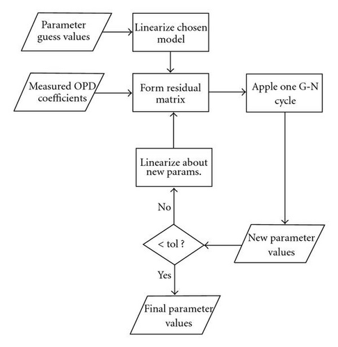
To minimize the error measure Δ² and hence determine the most likely shape of the mirror, we employed an iterative generalized Guass-Newtom optimization that starts with guess values for the mirror shape parameters (radius of curvature and conic constant) and iteratively finds the minimum value of Δ². This algorithm requires Z to be linearized anew during each iteration of the regression about the values of the shape parameters θ found during the previous iteration. This is accomplished via the linear models of (11), (15), and (17) which are arrayed as in (18) in the expectation matrix H.

3.2. Construction of the Residual Matrix Z

Since our regression will proceed iteratively, we will use the linear models developed above. We perform three different regressions on our data, each based on the three models embodied in (11), (15), and (17). Recall the three models differ in how we treat possible misalignment of the mirror parent axes from the translation axes. First, we have to specify the experimental settings, or the translational misalignments that we introduce during each measurement. Then, we construct an expectation matrix H (the matrix of theoretical OPD coefficients specified up to the free shape parameters) according to model Equation (11), (15), or (17), depending on whether and how we treat small angle displacements of the translation axes with respect to the mirror axes.

Experimental settings {x_n} will consist of the set of known translations

applied to the test mirror in its aligned state. These settings are arrayed in a 3 × N matrix X in which the three rows correspond to translation directions x, y, and z and the N columns correspond to the N measurements performed. The expectation matrix H is then constructed via the linearized models of (11), (15), and (17) and application of the matrix of experimential translation settings X. Equation (22)) below corresponds to the case in which the translation axes are assumed to be orthogonal and coincident with the canonical axes of the mirror. The case in which the translation axes are assumed orthogonal but are allowed to displace, by small angles, from the lab axes is embodied in (23). Equation ((24) governs the case in which the translation axes are allowed to displace independently from the lab coordinate axes

()

The quantities measured under each of the N experimental settings will be the M coefficients in the expansion of the OPD, or translation-induced optical path difference, δW(x, y).

During measurement, the matrix X of translations is applied to the mirror and the resulting changes in the interferogram, in terms of the coefficients

in the expansions of the OPD functions {δW_n(x, y)}, are recorded. In practice, for the nth measurement, an interferogram is recorded in the aligned state, then the translation t_n is applied, another interferogram is taken, and the difference in the two phase functions is calculated. This results in the difference OPD function δW_n(x, y). The M responses, or the coefficients in the Mth-order expansion of the OPD, are arrayed in the N rows of the N × M measurement matrix Y:

()

Note that the number of responses for each measurement is equal to the number of OPD expansion coefficients we wish to consider in our regression. If we had instead chosen to retain OPD data sets in the form of the raw interferometer output, then our measurements would each contain some tens of thousands of responses, one for each detector in the camera, and we would have to deal with this large data set at each iteration of the regression.

To begin the regression, we form the residual, matrix Z = Y − H. It is this residual matrix that represents the difference between the OPD coefficients that we measure and the theoretical coefficients which contain the free parameters. The estimated values for the true surface parameters θ will be obtained by minimizing, in the manner described above in Section 3.2, the residuals, according to the determinant criterion Δ² = |Z^TZ| of (21). That is, in each of the three cases embodied in (22), (23), (24), the free parameters are varied until the expectation functions fit the data optimally, so that the parameter estimation criterion Δ² is minimized.

The optimization algorithm is illustrated in the flowchart of Figure 1.

Details are in the caption following the image — **Figure 1**
Open in figure viewer PowerPoint

Flowchart for the multiresponse regression algorithm.

4. Application of Measurement Method to an Off-Axis Parabola

We tested our method using an off-axis parabola with known radius of curvature R = 304.8 mm, diameter D = 76.18 mm, and pupil offset s = −89.40 mm.

4.1. Experimental Setup

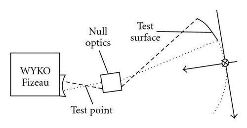
For our measurements, we used a WYKO 400 phase shifting interferometer with an f/3.4 transmission sphere and an inexpensive refractive null corrector we designed using COTS lenses. Translational motion was provided by three Newport DM-13 series manual differential micrometers with a resolution of 0.5 μm.

The mirror was mounted so that its parent optical axis coincided with the optical axis of the null corrector and the axes of translation coincided nominally with the home axes of the parent parabola. That is, the plane defined by the x and y axes of translation was parallel to the plane tangent to the parent vertex of the parabola and the z axis of translation was normal to the same plane. The image was centered on the detector plane of the interferometer by rotating about the test point as shown in Figure 2.

4.2. Model Functions

The surface altitude function from which we derived the model functions is the general conic of rotation with pupil offset s,

()

From this function, the components n_x(x, y), n_y(x, y), and n_z(x, y) of the surface normals are calculated and linearized about the nominal values R = 304.8 mm, K = −1, and s = −89.40 mm. The pupil coordinates are normalized to the pupil radius of 38.09 mm. Integrations are performed, using the orthonormal standard Zernikes as a basis, to obtain the OPD expansion coefficients and produce the matrix M, which transforms the vector

of translational components into the vector b of OPD expansion coefficients as described in (13). For these nominal values, considering the first five Zernike terms (excluding piston), the zeroth order matrix M⁽⁰⁾, in units of waves per micron, was calculated to be

()

In this matrix, the first, second, and third columns correspond to translations in the x, y, and z directions, respectively. Rows correspond to the first five standard Zernikes, beginning with x tilt (piston is excluded).

The presence of zero elements in the matrix M⁽⁰⁾ is due to the bilateral symmetry of the mirror about the x-z plane. Translations parallel to a plane of symmetry only produce aberrations with the same symmetry, and translations normal to a plane of symmetry do not produce any aberrations that are symmetric about that plane.

4.3. Imaging Distortion Compensation

The circular pupil of the off-axis parabola was distorted by the null corrector in such a way that it appeared oblong at the image plane of the interferometer. This presented a problem for the measurement, since the theory on which the regression is based requires that the OPD recorded by each detector in the array be associated with its true pupil coordinate. If we had not corrected for the distortion and just applied a circular analysis mask, then the Zernike decomposition would be distorted and the model functions would be inaccurate.

To correct for pupil image distortion, a procedure was employed which the authors have elaborated in a previously published paper [11]. In this procedure, fiducial mask features, whose locations in the physical pupil coordinates of the mirror are known beforehand, are imaged by the optical train comprising the interferometer and null corrector. Then a transformation is calculated that carries the pixel addresses of data points in the interferometer output into physical coordinates in the pupil of the mirror.

4.4. Zernike Decomposition

At each iteration of the multiresponse regression, the Zernike decomposition of the linearized model functions is performed numerically. In contrast, the raw data supplied by the interferometer need only to be decomposed into Zernike components once, at the beginning of the regression. This decomposition is accomplished by minimizing the variance between the data and a linear combination of sampled basis functions.

To take a measurement, we recorded an interferogram with the mirror aligned, and let its Zernike decomposition be b_M, and record another with the mirror in a translated position, and call its decomposition . The difference is the Zernike decomposition of the OPD function δW(x, y). This difference vector comprises the multiresponse result of a single measurement and forms one row of the data matrix Y.

We took five sets of measurements, each set containing three series of data, one for x translations, one for y translations and one for z translations. Each series involved translating the mirror in the corresponding direction from 5 μm to 50 μm in steps of 5 μm and from −5 μm to −50 μm in steps of −5 μm, for a total of twenty translations. Each measurement set, therefore, consisted of a total of 60 measurements, so that 300 measurements were taken in total.

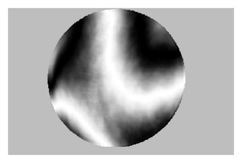
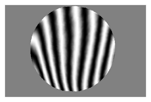
Two sample OPD maps are shown below in Figure 3. Figure 3(a) depicts the phase difference between the test mirror and the reference with the mirror in the aligned state and indicates null errors of about 1.528 waves. Figure 3(b) shows the interferogram when the mirror is translated 25 μm in the positive x direction (horizontal in the plots). The peak-to-valley phase difference in this state is 8.379 waves. The difference in the OPD coefficient vectors of the two maps comprises a single measurement. Figure 4 shows sample results for measurement of x tilt, y tilt, and focus components of the OPD as functions of x and y translations.

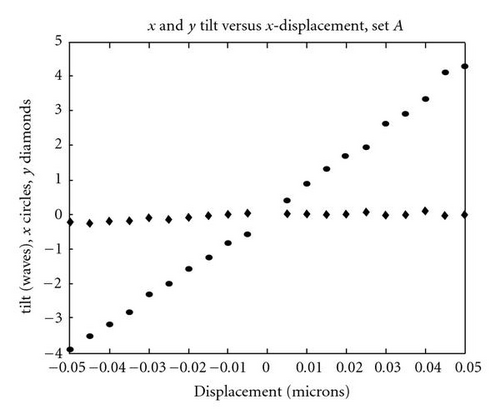
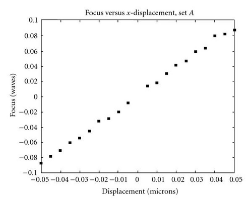
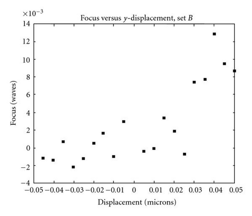
We see in the above figures that the mirror symmetry has had its predicted effect, however, the contribution to the translation induced wavefront aberration from components that should be zero, by symmetry arguments, is not quite zero due to mechanical errors. It is also important to note that the maximum displacement introduced to the mirror was kept within certain bounds (calculated based on a relationship derived in earlier, published work by the authors [3]) in order to prevent retrace error from confounding the measurements. The tell-tale sign of retrace errors would be a nonlinearity in the OPD coefficients as a function of displacement, which does not show up here.

4.5. Regression of R and K

After data are Zernike decomposed and the data matrix H is formed, the result is fed into the regression algorithm, the output of which consists of values for the radius of curvature R and conic constant K. We performed our regression using Matlab. The iteration proceeds until the magnitude of the increment vector δθ was less than 0.001.

In performing the regression, we found that the algorithm was most stable when we only considered the tilt and focus coefficients (i.e., coefficients one through three) in the Zernike expansions of the OPD. The other coefficients were small enough, that, when we retained them, the residual matrix was badly scaled. In other words, the columns of the residual matrix corresponding to the higher order Zernike polynomials were very small (close to zero) compared to the lower order columns. The more Zernike terms we included, the closer the residual matrix came to column rank deficiency and the more unstable the algorithm became. As discussed below, this simplification, in addition to being necessary, supplied reasonable, stable answers, and so it is justified on the grounds of correctness and economy. The reader can also be assured based on earlier work by Young and Dente [12] that the tilt coefficients as a function of translations of the mirror are indeed sensitive to conic constant.

4.6. Measurement Results

We applied the three regression algorithms corresponding to three models to three different cases, for a total of nine final measurement results. The three cases to which we applied the regression corresponded to three different ways that the data were conditioned before being sent to the regression algorithm. In the first case, all three hundred data points were used; in the second case, five aberrant data points were first removed; and in the third case, the aberrant data points were excluded and, in addition, the OPD coefficients that should have been zero, by the symmetry arguments presented in Section 4.2, were artificially zero. The argument for the validity of conditioning the data in the latter way is that the small angle dislocation of a translation axis will not affect the magnitude of the translation along the original, undisplaced axis. Therefore, it is valid to only consider OPD coefficients that should arise from translations along the undisplaced axis and to ignore OPD coefficients that should remain zero.

The results of our measurement are listed in Table 1 below. All the regressions supplied reasonable answers, except those in which the x and z axes were allowed to skew independently. In those cases, the vertex radius of curvature is found to be larger than the value specified by the manufacturer by around a centimeter, and the conic is found to be significantly closer to zero than its nominal value of −1. The angular displacements of the translation axes calculated using the second algorithm, where these axes are assumed orthogonal, were usually on the order of milliradians and in only a couple of cases were as large as one-hundredth radian. The third algorithm, on the other hand, always calculated a large value (negative one-fifth radian or ~11 degrees) for the angular displacement of the x translation axis about the y axis. This constitutes an unreasonably large skewing of the x and z axes and accounts for the departures of the calculated R and K for this case from reasonable values. Apparently, in these cases the algorithm is rather unstable and sees the mirror as a slower, less eccentric surface being translated along skewed axes.

Table 1. Results of measurement.

Algorithm	Data removed?	Symmetry zeroing?	Average R/K	RMS R/K	% Diff. R/K
1	N	N	304.3/−1.030	1.0/0.028	0.16/3.00
2	N	N	304.5/−1.023	1.7/0.040	0.10/2.30
3	N	N	316.2/−0.743	1.3/0.061	3.74/25.7
1	Y	N	304.1/−1.031	1.0/0.027	0.23/3.10
2	Y	N	304.6/−1.026	1.6/0.042	0.07/2.60
3	Y	N	314.5/−0.762	2.5/0.074	3.18/23.8
1	Y	Y	305.3/−1.025	2.7/0.032	0.16/2.50
2	Y	Y	305.3/−1.024	2.7/0.040	0.16/2.40
3	Y	Y	317.1/−0.659	6.9/0.271	4.04/34.1

The results that were closest to the specifications given by the manufacturer of R = 304.8 mm and K = −1 are obtained via the second algorithm, in which the orientation of the stage coordinate system is allowed to vary while the stage axes remain orthogonal. With the five aberrant data points removed, the answer for the vertex radius of curvature is slightly closer to 304.8, while the answer for the conic is slightly farther from its nominal value. In all cases, the values calculated for R are more precise (when the RMS deviation is normalized) than those calculated for K.

To examine the effect that different starting values have on the outcome of the regression, and to allay any concern that the algorithm trivially reproduces the guess values, we started with the values 335 mm for R and −1.1 for K, and only considered the cases, as shown below in Table 2, in which neither symmetry zeroing nor independent displacements of the translation axes were considered. For the two cases in which no displacements of the translation axes were considered at all, the answers were exactly the same for these new starting points. For the two in which the axes were allowed to displace as a whole while remaining orthogonal, the answers were slightly different with the answers for R departing more from the previous answers than the answers for K. The sensitivity of the algorithm to the starting points is low, especially considering that these starting points are far from reasonable, as they are a full 10% different from the nominal mirror parameters.

Table 2. Results of measurement using different starting values for R and K.

Algorithm	Data removed?	Zeroing?	Avg. R/K	RMS R/K	%Diff. R/K
1	N	N	304.3/−1.030	1.0/0.029	0.16/3.00
2	N	N	304.7/−1.022	1.7/0.039	0.03/2.30
1	Y	N	304.1/−1.031	1.0/0.027	0.23/3.10
2	Y	N	305.1/−1.027	1.3/0.041	0.10/2.70

4.7. Errors

If, as in (9) and (10), we expand the slopes of the OPD expansion coefficients to first order in R and K, we find that the K coefficients are always an order of magnitude or more larger than the R coefficients for our parabolic mirror. This indicates that the measured OPD is more sensitive to changes in K than to changes in R and that, inversely, K is less sensitive to errors in measurements of OPD than is R. The results of measurement bear this out, as the numerical values for the standard deviations and absolute errors are much smaller for K than for R. However, when the RMS is normalized to the nominal values of R and K, we find that the relative precision is much better for R than for K, since the nominal value of R is larger by a factor of about 300 than the magnitude of the nominal conic constant. The percent difference from the manufacturer’s metrology shows that the relative agreement in the measured value of R is indeed closer to the manufacturer’s values than is the measured value of K. The manufactured tolerance for R is +/−0.1% and the tolerance on K (calculated from the slope error tolerance) is 0.01%.

The precision and accuracy in the answers supplied by algorithms two and three suffer from the inclusion of more free parameters. This imprecision is minimal for algorithm two, but algorithm three drives the errors to intolerable levels. Merely removing five bad data points out of three hundred causes a large change in the answers and in the errors produced by the third algorithm. This demonstrates the numerical instability introduced by the included additional parameters in algorithm three.

Possible sources of error are errors in magnitudes of displacement as well as unaccounted for rotations due to moments applied to the stage when the micrometer knobs are turned. The random departure of the relationship between OPD and displacement from linearity indicates errors of the former kind, while the presence of significant Zernike components that should be disallowed by mirror symmetries indicates errors of the second kind.

To analyze errors introduced by coupling between translations and rotations, we examined the calculated radius and conic values for the case in which the orientation of the translation axes was allowed to vary, yet it remains orthogonal. The results for this case included, in addition to radius and conic values, the estimated rotations of the mirror coordinate system about the x,y, and z axes. We calculated the difference in regressed radius and conic values between the baseline case (with no presumed dislocation of the translation axes) and the aforementioned case, for all five measurement runs. (Note that the baseline case and the displaced case use, as they must, the same raw measurement data and only differ in the regression used to calculate radius and conic.) This resulted in an overdetermined system of equation from which the best fit error gains (which relate magnitudes of x, y, and z rotations of the system of translation axes to variations in regressed radius and conic values) were calculated via the pseudoinverse. Sensitivities of radius and conic to each type of mirror coordinate frame rotation are represented by these results. The error gains for rotations of the system of translation axes about the x, y, and z axes with respect to the calculated radius of curvature were −77, 39, and 102 (mm/radian), respectively. The corresponding gains for the conic constant were −0.76, −2.23, and 2.02 (radian⁻¹). These results suggest that measurement of the radius of curvature with this method is most sensitive to rotations of the system of translation axes about the x and z axes, whereas the conic measurement is most sensitive to rotations about the y and z axes.

Another possible source of error comes from the imaging distortion produced by the interferometer-null combination. The measured Zernikes coefficients and, therefore, the regressed radius and conic values are subject to errors in registration of the pixels of OPD data to coordinates in physical space. A thorough, quantitative study of this relationship will be left for future work for the sake of brevity but it should be noted that this distortion compensation process was fully reported in an earlier paper in this journal [11]. In that work, we concluded that our distortion correction method produced mapping errors that were less than a single pixel in the interferogram. For this reason, we consider the errors introduced here by the imaging distortion to be negligible compared to those introduced by the mechanical errors.

Since this method requires data being taken at a number of alignment positions, it is likely that significant OPD may be induced. In some intereferometers, and especially in combination with null optics, retrace error may confound the measurements by producing alignment sensitive errors in the measurement. This error can be ameliorated by empirical measurement of the retrace error sensitivity of the interferometric system, modeling of the null system according to previously published work by the coauthors [13], and by constraining the alignments to ranges which contribute sufficiently small errors. However, in precision optical testing, especially of large, lightweight mirrors that suffer significant gravity sag, these issues are typically already monitored and documented. Thus, this method does not require significant modifications or additions to standard interferometric testing procedures of hardware. The introduction of significant retrace error begins when the linearity of the approximate governing relationship of (3) breaks down. We have thoroughly analyzed these limits, based on the accuracy of the interferometer and the geometry of this particular test mirror, in another journal article [3] and used this analysis to bound the magnitude of displacements introduced during our test to 50 μm. Given the lack of systematic departure from linearity in the data and the thorough upfront analysis of the proper bounds for the mechanical displacements, we do not consider retrace error to be significant in this test, even though the OPD that we were able to induce is significant (several waves).

Environmental and instrumental errors such as air turbulence (which was mitigated by the placement of a cardboard box over the airpath) and errors introduced by finite accuracy of the interferometer are likely overwhelmed by the mechanical contributions to error that were discussed above. The OPD measurement accuracy of the WYKO 400 interferometer is on the order of λ/100, which is very small compared to the variations in measured OPD values.

It is important to note one source of error to which our method is highly insensitive: null errors. Since our method is differential in nature, the mild errors in the null are subtracted out during each measurement.

5. Summary and Conclusion

We have presented an elegant, flexible method for measuring the prescription of mirrors of any nominal shape, which is insensitive to null wavefront and alignment errors. Development of this method involved identifying the fundamental requirement that the testing be performed in a differential interferometric modality; realizing that the most elegant way to implement this differential measurement scheme was by introducing rigid body motions through a mechanical support that is already common in interferometric test setups and, perhaps most importantly, developing a sophisticated yet economical regression algorithm, based on the correct assumptions about the statistics of the measurement errors. We have successfully employed a method for measuring the prescription of an aspheric mirror using only the usual equipment necessary for performing interferometric figure tests. The method is suited to arbitrary mirror prescriptions and can be used in the conjugate null and center-of-curvature null test configuration. Such a method is suitable for the profile testing of reflective optics in a cryogenic testing situation, such as that encountered in James Webb Space Telescope testing, since it is a remote method and requires no more equipment than is necessary in making basic figure measurements.

With our setup, we were able to achieve vertex radius of curvature measurement accuracy of better than 0.1% and conic constant accuracy of better than 3% relative to the manufacturers measured values on an off-axis paraboloid with over X waves of deformation from a sphere, using a null assembled from COTS lenses.

The accuracy of our measurement technique would no doubt be greatly improved by enhancing the mechanical support for the mirror and using more accurate motion control. An electronically controlled translation stage, like those used in most cryogenic tests, would reduce the amount of extraneous mechanical movements of the mirror and would provide better translation accuracy and relief from backlash, especially if the magnitudes of the translations were monitored with distance measuring interferometers. Future work toward improving this method of shape measurement should concentrate on two general areas: improvement of mechanical support and motion induction and improvement of data acquisition. More accurately controlled movement, via, for example, the introduction of distance measuring interferometers to the translation stage, would reduce the amount of data that would have to be taken in order to achieve good accuracy and would reduce measurement time through automation. For in situ measurement of shape of a large optical surface in space, it would, of course, be necessary to move the interferometer head instead of the optic itself to obtain the differential measurements.

Acknowledgments

The authors would like to thank NASA Marshall Spaceflight Center and the National Science Foundation for funding portions of the work described here.

References

1 Chen F., Brown G. M., and Song M., Overview of three-dimensional shape measurement using optical methods, Optical Engineering. (2000) 39, no. 1, 10–22, 2-s2.0-0033895371, https://doi.org/10.1117/1.602438.
10.1117/1.602438
Web of Science® Google Scholar
2 Malacara J. Z., D. Malacara, Angle, distance, and focal length measurements, Optical Shop Testing, 1992, 2nd edition, John Wiley & Sons, New York, NY, USA, 715–741.
Google Scholar
3 Robinson B. M. and Reardon P. J., First-order perturbations of reflective surfaces and their effects in interferometric testing of mirrors, Journal of Modern Optics. (2005) 52, no. 18, 2625–2636, 2-s2.0-29744453709, https://doi.org/10.1080/09500340500260290.
10.1080/09500340500260290
CAS Web of Science® Google Scholar
4 Arfken G. B. and Weber H. J., Mathematical Methods for Physicists, 2001, Harcourt Academic.
Google Scholar
5 Bates D. M. and Watts D. G., Nonlinear Regression Analysis and Its Applications, 1988, John Wiley & Sons, New York, NY, USA.
10.1002/9780470316757
Google Scholar
6 Box G. E. P. and Tiao G. C., Bayesian Inference in Statistical Analysis, 1973, Addison-Wesley, Reading, Mass, USA.
Google Scholar
7 Gallant A. R., Nonlinear Statistical Models, 1987, John Wiley & Sons, New York, NY, USA.
10.1002/9780470316719
Google Scholar
8 Seber G. A. F. and Wild C. J., Nonlinear Regression, 1989, John Wiley & Sons, New York, NY, USA.
10.1002/0471725315
Google Scholar
9 Box G. E. P. and Draper N. R., The Bayesian estimation of common parameters from several responses, Biometrika. (1965) 52, 355–365.
10.1093/biomet/52.3-4.355
Web of Science® Google Scholar
10 Hunter W. G., Estimation of unknown constants from multiresponse data, Industrial and Engineering Chemistry Fundamentals. (1967) 6, no. 3, 461–463, 2-s2.0-33947335475.
10.1021/i160023a023
CAS Google Scholar
11 Robinson B. M. and Reardon P. J., Distortion compensation in interferometric testing of mirrors, Applied Optics. (2009) 48, no. 3, 560–565, 2-s2.0-61349166523, https://doi.org/10.1364/AO.48.000560.
10.1364/AO.48.000560
PubMed Web of Science® Google Scholar
12 Young E. W. and Dente G. C., The effects of rigid body motion in interferometric tests of large-aperture, off-axis, aspheric optics, 540, Proceedings of the Southwest Conference on Optics, 1985, 59–68, Proceedings of SPIE, 2-s2.0-0022184412.
Google Scholar
13 Geary J. and Reardon P., The interferometer as an imaging system, Proceedings of the 4th Annual Optical Conference and Workshop, Patrick Airforce Base, 2009.
Google Scholar

Citing Literature

All articles

Mirror Prescription Regression: A Differential Interferometric Technique

Abstract

1. Introduction

2. Development of the Model Functions

2.1. Misalignment-Induced Optical Path Difference (OPD)