Volume 2010, Issue 1 107857
Review Article
Open Access

Instantons, Topological Strings, and Enumerative Geometry

Richard J. Szabo

Corresponding Author

Richard J. Szabo

Department of Mathematics, Heriot-Watt University, Colin Maclaurin Building, Riccarton, Edinburgh EH14 4AS, UK hw.ac.uk

Maxwell Institute for Mathematical Sciences, Edinburgh, UK maxwell.ac.uk

Search for more papers by this author
First published: 23 June 2010
Citations: 22
Academic Editor: M. N. Hounkonnou

Abstract

We review and elaborate on certain aspects of the connections between instanton counting in maximally supersymmetric gauge theories and the computation of enumerative invariants of smooth varieties. We study in detail three instances of gauge theories in six, four, and two dimensions which naturally arise in the context of topological string theory on certain noncompact threefolds. We describe how the instanton counting in these gauge theories is related to the computation of the entropy of supersymmetric black holes and how these results are related to wall-crossing properties of enumerative invariants such as Donaldson-Thomas and Gromov-Witten invariants. Some features of moduli spaces of torsion-free sheaves and the computation of their Euler characteristics are also elucidated.

1. Introduction

Topological theories in physics usually relate BPS quantities to geometrical invariants of the underlying manifolds on which the physical theory is defined. For the purposes of the present article, we will focus on two particular and well-known instances of this. The first is instanton counting in supersymmetric gauge theories in four dimensions, which gives the Seiberg-Witten and Donaldson-Witten invariants of four-manifolds. The second is topological string theory, which is related to the enumerative geometry of Calabi-Yau threefolds and computes, for example, Gromov-Witten invariants, Donaldson-Thomas invariants, Gopakumar-Vafa BPS invariants, and key aspects of Kontsevich′s homological mirror symmetry conjecture.

From a physical perspective, these topological models are not simply of academic interest, but they also serve as exactly solvable systems which capture the physical content of certain sectors of more elaborate systems with local propagating degrees of freedom. Such is the case for the models we will consider in this paper, which are obtained as topological twists of a given physical theory. The topologically twisted theories describe the BPS sectors of physical models, and compute nonperturbative effects therein. For example, for certain supersymmetric charged black holes, the microscopic Bekenstein-Hawking-Wald entropy is computed by the Witten index of the relevant supersymmetric gauge theory. This is equivalent to the counting of stable BPS bound states of D-branes in the pertinent geometry, and is related to invariants of threefolds via the OSV conjecture [1].

From a mathematical perspective, we are interested in counting invariants associated to moduli spaces of coherent sheaves on a smooth complex projective variety X. To define such invariants, we need moduli spaces that are varieties rather than algebraic stacks. The standard method is to choose a polarization on X and restrict attention to semistable sheaves. If X is a Kähler manifold, then a natural choice of polarization is provided by a fixed Kähler two-form on X. Geometric invariant theory then constructs a projective variety which is a coarse moduli space for semistable sheaves of fixed Chern character. In this paper we will be interested in the computation of suitably defined Euler characteristics of certain moduli spaces, which are the basic enumerative invariants. We will also compute more sophisticated holomorphic curve counting invariants of a Calabi-Yau threefold X, which can be defined using virtual cycles of the pertinent moduli spaces and are invariant under deformations of X. In some instances the two types of invariants coincide.

An alternative approach to constructing moduli varieties is through framed sheaves. Then there is a projective Quot scheme which is a fine moduli space for sheaves with a given framing. A framed sheaf can be regarded as a geometric realization of an instanton in a noncommutative gauge theory on X [24] which asymptotes to a fixed connection at infinity. The noncommutative gauge theory in question arises as the worldvolume field theory on a suitable arrangement of D-branes in the geometry. In Nekrasov′s approach [5], the set of observables that enter in the instanton counting are captured by the infrared dynamics of the topologically twisted gauge theory, and they compute the intersection theory of the (compactified) moduli spaces. The purpose of this paper is to overview the enumeration of such noncommutative instantons and its relation to the standard counting invariants of X.

In the following we will describe the computation of BPS indices of stable D-brane states via instanton counting in certain noncommutative and q-deformations of gauge theories on branes in various dimensions. We will pay particular attention to three noncompact examples which each arise in the context of Type IIA string theory.
  • (1) D6-D2-D0 bound states in D6-brane gauge theory—These compute Donaldson-Thomas invariants and describe atomic configurations in a melting crystal model [6]. This also provides a solid example of a (topological) gauge theory/string theory duality. The counting of noncommutative instantons in the pertinent topological gauge theory is described in detail in [7, 8].

  • (2) D4-D2-D0 bound states in D4-brane gauge theory—These count black hole microstates and allow us to probe the OSV conjecture. Their generating functions also appear to be intimately related to the two-dimensional rational conformal field theory.

  • (3) D2-D0 bound states in D2-brane gauge theory—These compute Gromov-Witten invariants of local curves. Instanton counting in the two-dimensional gauge theory on the base of the fibration is intimately related to instanton counting in the four-dimensional gauge theory obtained by wrapping supersymmetric D4-branes around certain noncompact four-cycles C, and also to the enumeration of flat connections in Chern-Simons theory on the boundary of C. These interrelationships are explored in detail in [913].

These counting problems provide a beautiful hierarchy of relationships between topological string theory/gauge theory in six dimensions, four-dimensional supersymmetric gauge theories, Chern-Simons theory in three dimensions, and a certain q-deformation of two-dimensional Yang-Mills theory. They are also intimately related to two-dimensional conformal field theory.

2. Topological String Theory

The basic setting in which to describe all gauge theories that we will analyse in this paper within a unified framework is through topological string theory, although many aspects of these models are independent of their connection to topological strings. In this section, we briefly discuss some physical and mathematical aspects of topological string theory, and how they naturally relate to the gauge theories that we are ultimately interested in. Further details about topological string theory can be found in, for example, [14, 15], or in [16] which includes a more general introduction. Introductory and advanced aspects of toric geometry are treated in the classic text [17] and in the reviews [18, 19]. The standard reference for the sheaf theory that we use is the book [20], while a more physicist-geared introduction with applications to string theory can be found in the review [21].

2.1. Topological Strings and Gromov-Witten Theory

Topological string theory may be regarded as a theory whose state space is a “subspace” of that of the full physical Type II string theory. It is designed so that it can resolve the mathematical problem of counting maps
(2.1)
from a closed oriented Riemann surface Σg of genus g into some target space X. In the physical Type II theory, any harmonic map f, with respect to chosen metrics on Σg and X, is allowed. They are described by solutions to second-order partial differential equations, the Euler-Lagrange equations obtained from a variational principle based on a sigma-model. The simplification supplied by topological strings is that one replaces this sigma-model on the worldsheet Σg by a two-dimensional topological field theory, which can be realized as a topological twist of the original 𝒩 = 2 superconformal field theory. In this reduction, the state space descends to its BRST cohomology defined with respect to the 𝒩 = 2 supercharges, which naturally carries a Frobenius algebra structure. This defines a consistent quantum theory if and only if the target space X is a Calabi-Yau threefold, that is, a complex Kähler manifold of dimension dim (X) = 3 with trivial canonical holomorphic line bundle KX, or equivalently trivial first Chern class c1(X): = c1(KX) = 0. We fix a closed nondegenerate Kähler (1,1)-form ω on X.

The corresponding topological string amplitudes Fg have interpretations in compactifications of Type II string theory on the product of the target space X with four-dimensional Minkowski space 3,1. For instance, at genus zero the amplitude F0 is the prepotential for vector multiplets of 𝒩 = 2 supergravity in four dimensions. The higher genus contributions Fg, g ≥ 1 correspond to higher derivative corrections of the schematic form R2T2g−2, where R is the curvature and T is the graviphoton field strength. We will now explain how to compute the amplitudes Fg. There are two types of topological string theories that we consider in turn.

2.1.1. A-Model

The A-model topological string theory isolates symplectic structure aspects of the Calabi-Yau threefold X. It is built on holomorphically embedded curves (2.1). The holomorphic string maps f in this case are called worldsheet instantons. They are classified topologically by their homology classes
(2.2)
With respect to a basis Si of two cycles on X, one can write
(2.3)
where the Betti number b2(X) is the rank of the second homology group H2(X, ), and ni. Due to the topological nature of the sigma-model, the string theory functional integral localizes equivariantly (with respect to the BRST cohomology) onto contributions from worldsheet instantons.
The sum over all maps can be encoded in a generating function which depends on the string coupling gs and a vector of variables defined as follows. Let
(2.4)
be the complex Kähler parameters of X with respect to the basis Si. They appear in the values of the sigma-model action evaluated on a worldsheet instanton. For an instanton in curve class (2.3), the corresponding Boltzmann weight is
(2.5)
Then the quantum string theory is described by a genus expansion of the free energy
(2.6)
weighted by the Euler characteristic χ(Σg) = 2 − 2g of Σg, where the genus g contribution to the statistical sum is given by
(2.7)
and in this formula the classes β ≠ 0 correspond to worldsheets of genus g. The numbers Ng,β(X) are called the Gromov-Witten invariants of X and they “count”, in an appropriate sense, the number of worldsheet instantons (holomorphic curves) of genus g in the two-homology class β. They can be defined as follows.
A worldsheet instanton (2.1) is said to be stable if the automorphism group Aut(Σg, f) is finite. Let 𝔐g(X, β) be the (compactified) moduli space of isomorphism classes of stable holomorphic maps (2.1) from connected genus g curves to X representing β. This is the instanton moduli space onto which the path integral of topological string theory localizes. It is a proper Deligne-Mumford stack over which generalizes the moduli space 𝔐g of “stable” curves of genus g. While the dimension of 𝔐g is 3g − 3, the moduli space 𝔐g(X, β) is in general reducible and of impure dimension, as all possible stable maps occur. However, there is a perfect obstruction theory [22] which generically has virtual dimension
(2.8)
When X is a Calabi-Yau threefold, this integer vanishes and there is a virtual fundamental class [22]
(2.9)
in the degree zero Chow group. In this case, we define
(2.10)
and so the Gromov-Witten invariants give the “virtual numbers” of worldsheet instantons. One generically has Ng,β(X) ∈ due to the orbifold nature of the moduli stack 𝔐g(X, β). One can also define invariants by integrating the Euler class of an obstruction bundle over 𝔐g(X, β). There are precise recipes for computing the Gromov-Witten invariants Ng,β(X) for toric varieties X.

2.1.2. B-Model

The B-model topological string theory isolates complex structure aspects of the Calabi-Yau threefold X. It enumerates the constant string maps which send the entire surface Σg to a fixed point in X, and hence have trivial curve class β = 0. The Gromov-Witten invariants in this case are completely understood. There is a natural isomorphism
(2.11)
and the degree zero Gromov-Witten invariants Ng,0(X) involve only the classical cohomology ring H(X, ) and “Hodge integrals” over the moduli spaces of Riemann surfaces 𝔐g defined as follows.

There is a canonical stack line bundle 𝔏𝔐g with fibre over the moduli point [Σg], the cotangent space of Σg at some fixed point. We define the tautological class ψ to be the first Chern class of 𝔏, ψ : = c1(𝔏) ∈ H2(𝔐g, ). The Hodge bundle 𝔈𝔐g is the complex vector bundle of rank g whose fibre over a point Σg is the space of holomorphic sections of the canonical line bundle . Let λj∶ = cj(𝔈) ∈ H2j(𝔐g, ). A Hodge integral over 𝔐g is an integral of products of the classes ψ and λj.

Explicit expressions for Ng,0(X) for generic threefolds X are then obtained as follows. Let {γa} aA be a basis for H(X, ) (modulo torsion), and let D2A index the generators of degree two. Then one has
(2.12)
where the Hodge integral can be expressed in terms of Bernoulli numbers as
(2.13)
Note that c1(X) = 0 above when X is Calabi-Yau.
Thus we know how to compute everything in the B-model, and it is completely under control. Our main interest is thus in extending these computations to the A-model. In analogy with the above considerations, one can note that there is a natural forgetful map
(2.14)
and then reduce any integral over 𝔐g(X, β) to 𝔐g using the corresponding Gysin push-forward map π!. However, this is difficult to do explicitly in most cases. The Gromov-Witten theory of X is the study of tautological intersections in the moduli spaces 𝔐g(X, β). There is a string duality between the A-model and the B-model which is related to homological mirror symmetry.

2.2. Open Topological Strings

An open topological string in X is described by a holomorphic embedding f : Σg,hX of a curve Σg,h of genus g with h holes. A D-brane in X is a choice of Dirichlet boundary condition on these string maps, which ensures that the Cauchy problem for the Euler-Lagrange equations on Σg,h locally has a unique solution. They correspond to Lagrangian submanifolds L of the Calabi-Yau threefold X, that is, ω|L = 0. If Σg,h = σ1 ∪ ⋯∪σh, then we consider holomorphic maps such that
(2.15)
This defines open string instantons, which are labelled by their relative homology classes
(2.16)
If we assume that b1(L) = 1, so that H1(L, ) is generated by a single nontrivial one-cycle γ, then
(2.17)
where wi, i = 1, …, h, are the winding numbers of the boundary maps .
The free energy of the A-model open topological string theory at genus g is given by
(2.18)
where w = (w1, …, wh) and the numbers Nw,g,β(X) are called relative Gromov-Witten invariants. To incorporate all topological sectors, in addition to the string coupling gs weighting the Euler characteristics χ(Σg,h) = 2 − 2gh, we introduce an N × N Hermitean matrix V to weight the different winding numbers. This matrix is associated to the holonomy of a gauge connection (Wilson line) on the D-brane. Then, taking into account that the holes are indistinguishable, the complete genus expansion of the generating function is
(2.19)
The traces are computed by formally taking the limit N and expanding in irreducible representations R of the D-brane gauge group U().

2.3. Black Hole Microstates and D-Brane Gauge Theory

When X is a Calabi-Yau threefold, certain BPS black holes on X × 3,1 can be constructed by D-brane engineering. D-branes in X correspond to submanifolds of X equipped with vector bundles with connection, the Chan-Paton gauge bundles, and they carry charges associated with the Chern characters of these bundles. This data defines a class in the differential K-theory of X, which provides a topological classification of D-branes in X.

The microscopic black hole entropy can be computed by counting stable bound states of D0–D2–D4–D6 branes wrapping holomorphic cycles of X with the following configurations:
  • (i)

    D6-brane charge 𝒬6,

  • (ii)

    D4-branes wrapping an ample divisor

    (2.20)
    with respect to a basis of four-cycles Ci, i = 1, …, b4(X) = b2(X), of X,

  • (iii)

    D2-branes wrapping a two-cycle

    (2.21)

  • (iv)

    D0-brane charge 𝒬0.

These D-brane charges give the black hole its charge quantum numbers. If we consider large enough numbers of D-branes in this system, then they form bound states which become large black holes with smooth event horizons, that can be counted and therefore account for the microscopic black hole entropy. In this scenario, are interpreted as magnetic charges and as electric charges. The thermal partition function defined via a canonical ensemble for the D0 and D2 branes with chemical potentials , and a microcanonical ensemble for the D4 and D6 branes, is given by
(2.22)
where Ω is the degeneracy of BPS states with the given D-brane charges.
As we mentioned in Section 2.1., the closed topological string amplitudes Fg are related to supergravity quantities on Minkowski spacetime 3,1. The fact that the genus zero free energy F0 for topological strings on X is a prepotential for BPS black hole charges in 𝒩 = 2 supergravity determines the entropy SBH(p, q) of an extremal black hole as a Legendre transformation of F0, provided that one fixes the charge moduli by the attractor mechanism. The genus zero topological string amplitude F0 is a homogeneous function of degree two in the 𝒩 = 2 vector multiplet fields XI. The black hole entropy in the supergravity approximation is then
(2.23)
where the chemical potentials μI are determined by the charges pI and qI by solving the equation
(2.24)
Further analyses of the entropy of 𝒩 = 2 BPS black holes on 3,1 have been extended to higher genus and suggest the relationship
(2.25)
between the black hole partition function (2.22) and the topological string partition function
(2.26)
where the moduli on both sides of this equation are related by their fixing at the attractor point
(2.27)
The remarkable relationship (2.25) is called the OSV conjecture [1]. It provides a means of using the perturbation expansion of topological strings and Gromov-Witten theory to compute black hole entropy to all orders. Alternatively, although the evidence for this proposal is derived for large black hole charge, the left-hand side of the expression (2.25) makes sense for finite charges and in some cases is explicitly computable in closed form. It can thus be used to define nonperturbative topological string amplitudes, and hence a nonperturbative completion of a string theory.
In the following, we will focus on the computation of the black hole partition function (2.22). The fact that this partition function is computable in a D-brane gauge theory will then give a physical interpretation of the enumerative invariants of X in terms of black hole entropy. Suppose that we have a collection of Dp-branes wrapping a submanifold Mp+1X, with dim (Mp+1) = p + 1 and Chan-Paton gauge field strength F. D-branes are charged with respect to supergravity differential form fields, the Ramond-Ramond fields, which are also classified topologically by differential K-theory. Recall that such an array couples to all n-form Ramond-Ramond fields C(n) through anomalous Chern-Simons couplings
(2.28)
where is the string length. In particular, these couplings contain all terms
(2.29)
and so the topological charge chm() of a Chan-Paton gauge bundle Mp+1 on a Dp-brane is equivalent to D(p − 2m)-brane charge. A prominent example of this, which will be considered in detail later on, is the coupling For p = 3, this shows that the counting of D4-D0 brane bound states is equivalent to the enumeration of instantons on the four-dimensional part of the D4-brane in X. The remaining sections of this paper look at these relationships from the point of view of various BPS configurations of these D-branes. We will study the enumeration problems from the point of view of gauge theories on the D-branes in order of decreasing dimensionality, stressing the analogies between each description.

3. D6-Brane Gauge Theory and Donaldson-Thomas Invariants

In this section we will look at a single D6-brane (𝒬6 = 1) and turn off all D4-brane charges (). We will discuss various physical theories which are modelled by the D6-brane gauge theory in this case, but otherwise have no a priori relation to string theory. These will include a tractable model for quantum gravity and the statistical mechanics of certain atomic crystal configurations. From the perspective of enumerative geometry, these partition functions will compute the Donaldson-Thomas theory of X.

3.1. Kähler Quantum Gravity

We will construct a model of quantum gravity on any Kähler threefold X, which will motivate the sorts of counting problems that we consider in this section. The partition function is defined by
(3.1)
where
(3.2)
The sum is over “quantized” Kähler two-forms on X, in the following sense. We decompose the “macroscopic” form ω into a fixed “background” Kähler two-form ω0 on X and the curvature F of a holomorphic line bundle over X as
(3.3)
To satisfy the requirement that there are no D4-branes in X, we impose the fluctuation condition
(3.4)
for all two-cycles βH2(X, ).
Substituting (3.3) together with (3.4) into (3.2) gives the action
(3.5)
The statistical sum (3.1) thus becomes (dropping an irrelevant constant term)
(3.6)
where , , and chm() denotes the mth Chern character of the given line bundle X. Note the formal similarity with the A-model topological string partition function constructed in Section 2.1. However, there is a problem with the way in which we have thus far set up this model. The fluctuation condition (3.4) on F implies ch2() = ch3() = 0. Hence only trivial line bundles can contribute to the sum (3.6), and the partition function is trivial.
The resolution to this problem is to enlarge the range of summation in (3.6) to include singular gauge fields and ideal sheaves. Namely, we take F to correspond to a singular U(1) gauge field A on X. This can be realized in two (related) possible ways:
  • (1)

    we can make a singular gauge field A nonsingular on the blow-up

    (3.7)
    of the target space, obtained by blowing up the singular points of A on X into copies of the complex projective plane 2. This means that the quantum gravitational path integral induces a topology change of the target space X. This is referred to as “quantum foam” in [23, 24], or

  • (2)

    we can relax the notion of line bundle to ideal sheaf. Ideal sheaves lift to line bundles on . However, there are “more” sheaves on X than blow-ups of X.

In this paper we will take the second point of view. Recall that torsion-free sheaves on X can be defined by the property that they sit inside short exact sequences of sheaves of the form
(3.8)
where is a holomorphic vector bundle on X, and 𝒮Z is a coherent sheaf supported at the singular points ZX of a gauge connection A of . Applying the Chern character to (3.8) and using its additivity on exact sequences give
(3.9)
for each m. Thus torsion-free sheaves fail to be vector bundles at singular points of gauge fields, and including the singular locus can reinstate the nontrivial topological quantum numbers that we desired above.

As we will discuss in detail in this section, this construction is realized explicitly by considering a noncommutative gauge theory on the target space X = 3. We will see that the instanton solutions of gauge theory on a noncommutative deformation are described in terms of ideals in the polynomial ring [z1, z2, z3]. For generic X, the global object that corresponds locally to an ideal is an ideal sheaf, which in each coordinate patch UαX is described as an ideal in the ring of holomorphic functions on Uα. More abstractly, an ideal sheaf is a rank one torsion-free sheaf with c1() = 0. This is a purely commutative description, since the holomorphic functions on 3 form a commutative subalgebra of for the Moyal deformation that we will consider. Thus the desired singular gauge field configurations will be realized explicitly in terms of noncommutative instantons [23, 24].

3.2. Crystal Melting and Random Plane Partitions

As we will see, the counting of ideal sheaves is in fact equivalent to a combinatorial problem, which provides an intriguing connection between the Kähler quantum gravity model of Section 3.1. and a particular statistical mechanics model [6]. Consider a cubic crystal

image

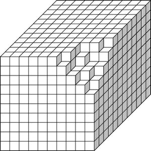
located on the lattice . Suppose that we start heating the crystal at its outermost right corner. As the crystal melts, we remove atoms, depicted symbolically here by boxes, and arrange them into stacks of boxes in the positive octant. Owing to the rules for arranging the boxes according to the order in which they melt, this configuration defines a plane partition or a three-dimensional Young diagram.

image

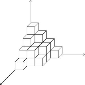
Removing each atom from the corner of the crystal contributes a factor q = eμ/T to the Boltzmann weight, where μ is the chemical potential and T is the temperature.

Let us define more precisely the combinatorial object that we have constructed, which generalizes the usual notion of partition and Young tableau. A plane partition is a semiinfinite rectangular array of nonnegative integers
(3.10)
such that πi,jπi+1,j, and πi,jπi,j+1 for all i, j ≥ 1. We may regard a partition π as a three-dimensional Young diagram, in which we pile πi,j cubes vertically at the (i, j)th position in the plane as depicted above. The volume of a plane partition
(3.11)
is the total number of cubes. The diagonal slices of π are the partitions (πi,i+m) i≥1, m ≥ 0, obtained by cutting the three-dimensional Young diagram with planes, and they represent a sequence of ordinary partitions (Young tableaux) λ = (λ1, λ2, …), with λiλi+1 for all i ≥ 1. Here λi ≥ 0 is the length of the ith row of the Young diagram, viewed as a collection of unit squares, and only finitely many λi are nonzero.
The counting problem for random plane partitions can be solved explicitly in closed form. For this, we consider the statistical mechanics in a canonical ensemble in which each plane partition π has energy proportional to its volume |π|. The corresponding partition function then gives the generating function for plane partitions
(3.12)
where pp(N) is the number of plane partitions π with |π | = N boxes. The function M(q) is called the MacMahon function.

3.3. Six-Dimensional Cohomological Gauge Theory

We will now describe a U(1) gauge theory formulation of the above statistical models [7, 8, 24]. If we gauge-fix the residual symmetry of the quantized Kähler gravity action (3.5), we obtain the action
(3.13)
where dA = d −   i  [A, −] is the gauge covariant derivative acting on the complex scalar field Φ, ⋆ denotes the Hodge operator with respect to the Kähler metric of X, and F = dA is the curvature two-form which has the Kähler decomposition F = F2,0 + F1,1 + F0,2. The field theory defined by this action arises in three (related) instances such as:
  • (1)

    a topological twist of maximally supersymmetric Yang-Mills theory in six dimensions,

  • (2)

    the dimensional reduction of supersymmetric Yang-Mills theory in ten dimensions on X,

  • (3)

    the low-energy effective field theory on a D6-brane wrapping X in Type IIA string theory, with D2 and D0 brane sources.

The gauge theory has a BRST symmetry [25, 26] and its partition function localizes at the BRST fixed points described by the equations
(3.14)
(3.15)
(3.16)
These equations also describe three (related) quantities:
  • (i)

    the Donaldson-Uhlenbeck-Yau (DUY) equations expressing Mumford-Takemoto slope stability of holomorphic vector bundles over X with finite characteristic classes,

  • (ii)

    BPS solutions in the gauge theory which correspond to (generalized) instantons,

  • (iii)

    bound states of D0–D2 branes in a single D6-brane wrapping X.

Recall that (3.14) and (3.15) are a special instance of the Hermitean Yang-Mills equations in which a constant λ is added to the right-hand side of (3.15). These equations arise in compactifications of heterotic string theory. The condition that the compactification preserves at least one unbroken supersymmetry requires λ = 0. These are the natural BPS conditions on a Kähler manifold (X, ω0) which generalize the usual self-duality equations in four dimensions.

The localization of the gauge theory partition function Z onto the corresponding instanton moduli space 𝔐X can be written symbolically as [24, 26]
(3.17)
where e(𝔑X) is the Euler class of the obstruction bundle 𝔑X whose fibres are spanned by the zero modes of the antighost fields. The zero modes of the fermion fields in the full supersymmetric extension of (3.13) [25, 26] are in correspondence with elements in the cohomology groups of the twisted Dolbeault complex
(3.18)
with ad  𝒫 the adjoint gauge bundle over X. By incorporating the gauge fields, one can rewrite this complex in the form [24]
(3.19)
which describes solutions of the DUY equations up to linearized complex gauge transformations. The morphism Ω0,3(X, ad  𝒫) → Ω0,2(X, ad  𝒫) here is responsible for the appearance of the obstruction bundle in (3.17) [24, 26].

In order for the integral (3.17) to be well defined, we need to choose a compactification of 𝔐X. In light of our earlier discussion, we will take this to be the Gieseker compactification, that is, the moduli space of ideal sheaves on X. The corresponding variety 𝔐X stratifies into components Hilbn,β(X) given by the Hilbert scheme of points and curves in X, parameterizing isomorphism classes of ideal sheaves with ch1() = c1() = 0, ch2() = −β, and ch3() = −n. The partition function (3.17) is the generating function for the number of D0-D2 brane bound states in the D6-brane wrapping X. Mathematically, these are the Donaldson-Thomas invariants of X. We will define this moduli space integration, and hence these invariants, more precisely in Section 3.9.

3.4. Localization in Toric Geometry

Toric varieties provide a large class of algebraic varieties in which difficult problems in algebraic geometry can be reduced to combinatorics. Much of this paper will be concerned with these geometries as they possess symmetries which facilitate computations, particularly those involving moduli space integrations. Let us start by recalling some basic notions from toric geometry. Below we give the pertinent definitions specifically in the case of varieties of complex dimension three, the case of immediate interest to us, but they extend to arbitrary dimensions in the obvious ways.

A smooth complex threefold X is called a toric manifold if it densely contains a (complex algebraic) torus T3 and the natural action of T3 on itself (by translations) extends to the whole of X. Basic examples are the torus T3 itself, the affine space 3, and the complex projective space 3. If in addition X is Calabi-Yau, then X is necessarily noncompact.

One of the great virtues of working with toric varieties X is that their geometry can be completely described by combinatorial data encoded in a toric diagram. The toric diagram is a graph consisting of the following ingredients:
  • (i)

    a set of vertices f which are the fixed points of the T3-action on X, such that X can be covered by T3-invariant open charts homeomorphic to 3,

  • (ii)

    a set of edges e which are T3-invariant projective lines 1X joining particular pairs of fixed points f1, f2,

  • (iii)

    a set of “gluing rules” for assembling the 3 patches together to reconstruct the variety X. In a neighbourhood of each edge e, X looks like the normal bundle over the corresponding 1. Since this normal bundle is a holomorphic bundle of rank two and every bundle over 1 is a sum of line bundles (by the Grothendieck-Birkhoff theorem), it is of the form

    (3.20)
    for some integers m1, m2. The normal bundle in this way determines the local geometry of X near the edge e via the transition function
    (3.21)
    between the corresponding affine patches (going from the north pole to the south pole of the associated 1). In the Calabi-Yau case, the Chern numbers c1(X) = 0 and c1(1) = 2 imply the condition m1 + m2 = 2.

For an open toric manifold X, we can exploit the toric symmetries to regularize the infrared singularities on the instanton moduli space 𝔐X by “undoing” the T3-rotations by gauge transformations [5]. In this way we will compute our moduli space integrals by using techniques from equivariant localization, which in the present context will be refered to as toric localization. Recall that the bosonic sector of the topologically twisted theory comprises a gauge connection Ai and a complex Higgs field Φ. In particular, the supercharges contain a scalar Q and a vector Qi. Generically, only Q is conserved and can be used to define the topological twist of the gauge theory. If the threefold X has symmetries then one can also use Qi. In the generic formulation of the theory, one only considers the scalar topological charge Q and restricts attention to gauge-invariant observables. But in the present case one can also use the linear combination
(3.22)
where ϵa are the parameters of the isometric action of T3U(3) on the Kähler space 3, and are vector fields which generate SO(6) rotations of 36. In this case we also consider observables which are only gauge-invariant up to a rotation. This means that the new observables are equivariant differential forms and the BRST charge QΩ can be interpreted as an equivariant differential d + ιΩ on the space of field configurations, where ιΩ acts by contraction with the vector field Ω.
This procedure modifies the action and the equations of motion by mixing gauge invariance with rotations. This set of modifications can sometimes be obtained by defining the gauge theory on an appropriate supergravity background called the “Ω-background”. In particular, the fixed point equation (3.16) is modified to
(3.23)
The set of equations (3.14), (3.15), and (3.23) minimizes the action of the cohomological gauge theory in the Ω-background and describes T3-invariant instantons (or, as we will see, ideal sheaves). In particular, there is a natural lift of the toric action to the instanton moduli space 𝔐X. We will henceforth study the gauge theory equivariantly and interpret the truncation of the partition function (3.17) as an equivariant integral over 𝔐X. This will always mean that we work solely in the Coulomb branch of the gauge theory. Due to the equivariant deformation of the BRST charge, these moduli space integrals can be computed via equivariant localization.

3.5. Equivariant Integration over Moduli Spaces

We now explain the localization formulas that will be used to compute partition functions throughout this paper. Let 𝔐 be a smooth algebraic variety. Then we can define the -equivariant cohomology as the ordinary cohomology of the Borel-Moore homotopy quotient , where is a contractible space on which acts freely. In the present example of interest, N = 1 and k = 3. Given a -equivariant vector bundle 𝔈𝔐, the quotient is a vector bundle over . The -equivariant Euler class of 𝔈 is the invertible element defined by
(3.24)
where e is the ordinary Euler class for vector bundles (the top Chern class).

Let Then is a universal principal -bundle, and there is a fibration with fibre 𝔐. Integration in equivariant cohomology is defined as the pushforward ∮𝔐 of the collapsing map 𝔐 → pt, which coincides with integration over the fibres 𝔐 of the bundle in ordinary cohomology. Let for i = 1, …, k and let ql :  for l = 1, …, N be the canonical projections onto the ith and lth factors. Introduce equivariant parameters , with and , with .

The Atiyah-Bott localization formula in equivariant cohomology states that
(3.25)
for any equivariant differential form , where the complex vector bundle is the normal bundle over the (compact) fixed point submanifold in 𝔐. When consists of finitely many isolated points f, this formula is simplified to
(3.26)
Each term in this sum takes values in the polynomial ring
(3.27)
in the generators of . When the manifold 𝔐 is noncompact, integration along the fibre is not a well-defined -linear map. Nevertheless, when is compact, we can formally define the equivariant integral ∮𝔐α by the right-hand side of the formula (3.25).
Going back to our example, when X = 3, one has ch2() = 0 and the partition function Z is saturated by contributions from isolated, pointlike instantons (D0-branes) by a formal application of the localization formula (3.26). However, these expressions are all rather symbolic, as we are not guaranteed that the algebraic scheme 𝔐X is a smooth variety, that is, the instanton moduli space has a well-defined stable tangent bundle with tangent spaces all of the same dimension. However, the variety 𝔐X is generically smooth and there is a well-defined virtual tangent bundle. The moduli space integration (3.26) can then be formally defined by virtual localization in equivariant Chow theory. As discussed in [27], the (stratified components of the) instanton moduli space 𝔐X carries a canonical perfect obstruction theory in the sense of [22]. In obstruction theory, the virtual tangent space at a point [] ∈ 𝔐X is given by
(3.28)
where is the Zariski tangent space and the obstruction space of 𝔐X at []. Its dimension is given by the difference of Euler characteristics . The kernel of the trace map
(3.29)
is the obstruction to smoothness at a point [] of the moduli space.

The bundles , i = 1,2 for [] ∈ 𝔐X define a canonical Tk-equivariant perfect obstruction theory 𝔈 = (𝔈1𝔈2) (see [22, Section 1]) on the instanton moduli space 𝔐 = 𝔐X. In this case, one may construct a virtual fundamental class [𝔐] vir and apply a virtual localization formula. The general theory is developed in [22] and requires a Tk-equivariant embedding of 𝔐 in a smooth variety 𝔜. The existence of such an embedding in the present case follows from the stratification of 𝔐X into Hilbert schemes of points and curves. Then one can deduce the localization formula over 𝔐 from the known ambient localization formula over the smooth variety 𝔜, as above. In this paper we will only need a special case of this general framework, the virtual Bott residue formula.

We can decompose 𝔈i into Tk-eigenbundles. The scheme theoretic fixed point locus is the maximal Tk-fixed closed subscheme of 𝔐. It carries a canonical perfect obstruction theory, defined by the Tk-fixed part of the restriction of the complex 𝔈 to , which may be used to define a virtual structure on . The sum of the nonzero Tk-weight spaces of defines the virtual normal bundle 𝔑vir to . Define the Euler class of a virtual bundle 𝔄 = 𝔄1𝔄2 using formal multiplicativity, that is, as the ratio of the Euler classes of the two bundles, e(𝔄) = e(𝔄1)/e(𝔄2). Then the virtual Bott localization formula for the Euler class of a bundle 𝔄 of a rank equal to the virtual dimension of 𝔐 reads [22]
(3.30)
where the integration is again defined via pushforward maps. The equivariant Euler classes on the right-hand side of this formula are invertible in the localized equivariant Chow ring of the scheme 𝔐 given by , where [ϵ1, …, ϵk] 𝔪 is the localization of the ring [ϵ1, …, ϵk] at the maximal ideal 𝔪 generated by ϵ1, …, ϵk.
If 𝔐 is smooth, then is the nonsingular set theoretic fixed point locus, consisting here of finitely many points []. However, in general the formula (3.30) must be understood scheme theoretically, here as a sum over Tk-fixed closed subschemes of 𝔐 supported at the points (with k = 3). With  : , i = 1,2, denoting the induced torus actions on the tangent and obstruction bundles on 𝔐, one generically has decompositions
(3.31)
where is a Tk-invariant subspace of . As demonstrated in [27, Section 4.5], the kernel module in (3.31) vanishes. Hence each subscheme here is just the reduced point [] and the Tk-fixed obstruction theory at [] is trivial. Under these conditions, the virtual localization formula (3.30) may be written as
(3.32)
The right-hand side of this formula again takes values in the polynomial ring [ϵ1, …, ϵk]. When for all [] ∈ 𝔐X, the moduli space 𝔐X is a smooth algebraic variety with the trivial perfect obstruction theory and this equation reduces immediately to the standard localization formula in equivariant cohomology given above. In this paper, we will make the natural choice for the bundle 𝔄, the virtual tangent bundle Tvir𝔐 itself.

3.6. Noncommutative Gauge Theory

To compute the instanton contributions (3.17) to the partition function of the cohomological gauge theory, we have to resolve the small instanton ultraviolet singularities of 𝔐X. This can be achieved by replacing the space X = 36 with its noncommutative deformation defined by letting the coordinate generators xi,   i = 1, …, 6, satisfy the commutation relations of the Weyl algebra
(3.33)
where
(3.34)
is a constant 6 × 6 skew-symmetric matrix which we take in Jordan canonical form without loss of generality (by a suitable linear transformation of 6 if necessary). We will assume that θ1, θ2, θ3 > 0 for simplicity. The noncommutative polynomial algebra
(3.35)
is regarded as the “algebra of functions” on the noncommutative space .
We can represent the algebra 𝒜 on the standard Fock module
(3.36)
where the orthonormal basis states |i, j, k〉 are connected by the action of creation and annihilation operators and αa, a = 1,2, 3. They obey αa | 0,0, 0〉 = 0 and
(3.37)
In the Weyl operator realization with the complex combinations of operators
(3.38)
for a = 1,2, 3, derivatives of fields are replaced by the inner automorphisms
(3.39)
while spacetime averages are replaced by traces over according to
(3.40)
In the noncommutative gauge theory, we introduce the covariant coordinates
(3.41)
and their complex combinations
(3.42)
for a = 1,2, 3. Then the (1,1) and (2,0) components of the curvature two-form can be, respectively, expressed as
(3.43)
while the covariant derivatives of the Higgs field become
(3.44)
The instanton equations (3.14), (3.15), and (3.23) then become algebraic equations
(3.45)
These equations describe BPS bound states of the D0–D6 system in a B-field background, which is necessary for reinstating supersymmetry [28, 29]. In addition, T3-invariance of the (unique) holomorphic three-form on X imposes the Calabi-Yau condition
(3.46)

3.7. Instanton Moduli Space

A major technical advantage of introducing the noncommutative deformation is that the instanton moduli space can be constructed explicitly, by solving the noncommutative instanton equations (3.45). First we construct the vacuum solution of the noncommutative gauge theory, with F = 0. It is obtained by setting A = 0 and is given explicitly by harmonic oscillator algebra
(3.47)
Other solutions are found via the solution generating technique described in, for example, references [30, 31]. For the general solution, fix an integer n ≥ 1 and let Un be a partial isometry on the Hilbert space which projects out all states |i, j, k〉 with i + j + k < n. Such an operator satisfies the equations
(3.48)
where
(3.49)
is a Hermitean projection operator onto a finite-dimensional subspace of . Then we make the ansatz
(3.50)
where f is a real function of the number operator
(3.51)
Using standard harmonic oscillator algebra, we can write the DUY equations (3.45) as
(3.52)
This recursion relation has a unique solution with the initial conditions f(i) = 0, i = 0,  1, …, n − 1, and the finite energy condition f(r) → 1 as r. It is given by [32]
(3.53)
The topological charge of the corresponding noncommutative instanton is
(3.54)
Thus the instanton number is the number of states in with N < n, that is, the number of vectors removed by Un, or equivalently the rank of the projector Πn.
The partial isometry Un identifies the full Fock space with the subspace
(3.55)
where
(3.56)
is a monomial ideal of codimension = (n) in the polynomial ring [w1, w2, w3]. The instanton moduli space can thus be identified as the Hilbert scheme
(3.57)
of points in X = 3. The Hilbert-Chow morphism
(3.58)
identifies the Hilbert scheme of points as a crepant resolution of the (coincident point) singularities of the th symmetric product orbifold of X. The ideal defines a plane partition π with |π| = boxes given by
(3.59)
Heuristically, this configuration represents instantons which sit on top of each other at the origin of 3, and along its coordinate axes where they asymptote to four-dimensional noncommutative instantons at infinity described by ordinary Young tableaux λ.

3.8. Donaldson-Thomas Theory

We can finally compute the instanton contributions to the partition function of the cohomological gauge theory on any toric Calabi-Yau threefold X [7, 8, 24]. Let us start with the case X = 3. Using (3.54), the contribution of an instanton corresponding to a plane partition π contributes a factor
(3.60)
to the Boltzmann weight appearing in the functional integral. There is also a measure factor which comes from integrating out the bosonic and fermionic fields in the supersymmetric gauge theory. This yields a ratio of fluctuation determinants
(3.61)
with the normalized character
(3.62)
where we have used the solution for Φ in (3.50). Using the Calabi-Yau condition ϵ1 + ϵ2 + ϵ3 = 0, it is easy to see that these determinants cancel up to a sign.
After some computation, one can explicitly determine this sign to get
(3.63)
The contribution Z from the empty partition is the one-loop perturbative contribution to the functional integral, and hence will be dropped. Then the instanton sum for the partition function is given by
(3.64)
which is just the MacMahon function M(q) with . This is the known formula for the Donaldson-Thomas partition function on 3.
For later use, let us note a convenient resummation formula for this partition function [6]. Using interlacing relations, the sum over plane partitions π can be converted into a triple sum over the Young tableaux obtained from the main diagonal slice λ = (πi,i) i≥1, together with a sum over pairs of semistandard tableaux of shape λ obtained by putting m + 1 of them in boxes of the skew diagram associated to the mth diagonal slice for each m ≥ 0. The partial sum over each semistandard tableaux coincides with the combinatorial definition of the Schur functions at a particular value, which can be expressed through the hook formula
(3.65)
where n(λ) = ∑i(i − 1)λi, and h(i, j) is the hook length of the box located at position (i, j) in the Young tableau . Then the partition function can be rewritten as a sum over ordinary partitions
(3.66)

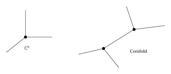
This construction can be generalized to arbitrary toric Calabi-Yau threefolds X by using the gluing rules of toric geometry. The two simplest such varieties are described by the toric diagrams

image

with a single vertex representing X = 3, whose partition function was computed above and is the basic building block for the generating functions on more complicated geometries, and a single line joining two vertices representing the resolved conifold , where the 1 contribute to the FFω0 term of the gauge theory action (3.13). The T3-invariant noncommutative U(1) instantons on X correspond to ideal sheaves and are described by the following combinatorial data:
  • (1)

    three-dimensional partitions πf at each vertex f of the toric diagram, corresponding to monomial ideals f[w1, w2, w3],

  • (2)

    two-dimensional partitions λe at each edge e of the toric diagram, representing the four-dimensional instanton asymptotics of πf.

This description requires generalizing the calculation on X = 3 above to compute the perpendicular partition function Pλ,μ,ν(q) [6], which is defined to be the generating function for three-dimensional partitions with fixed asymptotics λ, μ, and ν in the three coordinate directions. Such partitions correspond to instantons on with nontrivial boundary conditions at infinity along each of the coordinate axes. It can be expressed in terms of skew Schur functions, with .

For the example of the resolved conifold, using the gluing rules one easily computes
(3.67)
More generally, with these rules one finds that the instanton partition function is the generating function
(3.68)
for the Donaldson-Thomas invariants In,β(X) ∈ , which are defined as follows. The moduli variety Hilbn,β(X) of ideal sheaves on X is a projective scheme with a perfect obstruction theory. For general threefolds X, it has virtual dimension [33, Lemma 1]
(3.69)
which coincides with that of 𝔐g(X, β) from Section 2.1. In the Calabi-Yau case, the virtual dimension is zero, and the corresponding virtual cycle is
(3.70)
Then the Donaldson-Thomas invariants
(3.71)
count the virtual numbers of ideal sheaves on X with the given Chern character. The right-hand side is defined via equivariant integration, as explained in Section 3.5. The torus action on X lifts to the moduli scheme Hilbn,β(X). The -fixed locus has a -equivariant virtual theory with cycle and virtual normal bundle in the equivariant K-theory . This construction gives precise meaning to the moduli space integral (3.17) via application of the virtual localization formula in equivariant Chow theory, described in Section 3.5.

3.9. Wall-Crossing Formulas

We will now make contact with Section 2. For the present class of threefolds X, there is a gauge theory/string theory duality [27]. This follows from the fact that the perpendicular partition function Pλ,μ,ν(q) is related to the Calabi-Yau crystal formulation of the topological vertex
(3.72)
with which are the building blocks for the computation of the generating function for Gromov-Witten invariants using rules analogous to those described in Section 3.8 [14, 15]. Using these relations one can show that the six-dimensional cohomological gauge theory is S-dual to the A-model topological string theory. The respective partition functions are related by
(3.73)
where the Euler characteristic χ(X) of X is the number of vertices in its toric diagram. For the conifold example, the gluing rules for the topological vertex yield [14, 15]
(3.74)
which should be compared with (3.67). This Gromov-Witten/Donaldson-Thomas correspondence is known to hold for arbitrary toric threefolds [34]. The relationship (3.73) can be thought of as a wall-crossing formula, as we now explain.

The relationship (3.73) is in apparent contradiction with the OSV conjecture (2.25) if we wish to interpret the right-hand side as the generating function ZBH(1,0, ϕ2, ϕ0) of a suitable index for black hole microstates. However, the conjectural relations (2.25) and (3.73) hold in different regimes of validity. The number of BPS particles in four dimensions formed by wrapping supersymmetric bound states of D-branes around holomorphic cycles of X depends on the choice of a stability condition, and the BPS countings for different stability conditions are related by wall-crossing formulas. For example, stability of black holes requires that their chemical potentials μI lie in the ranges 𝒬0ϕ0 > 0 and .

On the other hand, the validity of (3.73) is related to the existence of BPS invariants Bg,β(X) ∈ such that the topological string amplitudes have an expansion given by [35, 36]
(3.75)
of which the conifold partition function (3.67) is an explicit case. These are partition functions of D6-D2-D0 brane bound states only for certain Kähler moduli. Analyses of Calabi-Yau compactifications of Type II string theory show that the Hilbert spaces of BPS states jump discontinuously across real codimension one walls in the moduli space of vacua, known as walls of marginal stability. The noncommutative instantons do not account for walls of marginal stability extending to infinity. One should instead apply some sort of stability condition (such as Π-stability) to elements of the bounded derived category of coherent sheaves Db(coh(X)) of the given charge, which gives a topological classification of A-model D-branes on X. These issues are discussed in more detail in [3739].

From a mathematical perspective, we can study this phenomenon by looking at framed moduli spaces, which consist of instantons that are trivial “at infinity”. More precisely, we can consider a toric compactification of X obtained by adding a compactification divisor D, and consider sheaves with a fixed trivialization on D. The Kähler polarization defined by ω0 allows us to define the moduli space of stable sheaves. Then the symbolic definition of the gauge theory partition function (3.17) as a particular Euler characteristic can be made precise in the more local definition of Donaldson-Thomas invariants given by [40].

As a scheme with a perfect obstruction theory, the instanton moduli space 𝔐X can be viewed locally as the scheme theoretic critical locus of a holomorphic function, the superpotential W, on a compact manifold 𝒳 with the action of a gauge group 𝒢. 𝔐X has virtual dimension zero, and at nonsingular points, the obstruction sheaf 𝔑X on 𝔐X coincides with the cotangent bundle. Hence if 𝔐X were everywhere nonsingular, then the partition function (3.17) would just compute the signed Euler characteristic . At singular points, however, the invariants differ from these characteristics.

There is a constructible function ν : 𝔐X which can be used to define the weighted Euler characteristic
(3.76)
For sheaves of fixed Chern character, this coincides with the curve-counting invariants In,β(X). At nonsingular points, , while at singular points it is the more complicated function given by
(3.77)
where MFW() is the Milnor fibre of the superpotential W at the point corresponding to . The weighted Euler characteristic is a deformation invariant of X.
In this approach, one can use topological Euler characteristics to define In,β(X) as invariants associated to moduli varieties of framed sheaves. Fixing βH2(X, ) and n, the variety Hilbn,β(X) equivalently parametrizes isomorphism classes of the following objects:
  • (a)

    surjections (framings)

    (3.78)
    with ch() = (1,0, β, n),

  • (b)

    stable sheaves with ch() = (1,0, −β, −n) and trivial determinant,

  • (c)

    subschemes SX of dimension ≤1 with curve class [S] = β and holomorphic Euler characteristic χ(𝒪S) = n.

The equivalences between these three descriptions are described explicitly for X = 3 in [7, 8].

As we vary the polarization ω0, the moduli spaces change and so do the associated counting invariants, leading to a wall-and-chamber structure. The wall-crossing behaviour of the enumerative invariants is studied in [41, 42]. The analog of varying ω0 for framed sheaves is to consider quotients of the structure sheaf 𝒪X in different abelian subcategories of the bounded derived category Db(coh(X)) of coherent sheaves on X. The analog of wall-crossing gives the Pandharipande-Thomas theory of stable pairs [43, 44] and the BPS invariants above. For this, the quotients of 𝒪X are the stable pairs (, α), where is a coherent 𝒪X-module of pure dimension one with ch2() = −β and χ() = −n, and α : 𝒪X is a nonzero sheaf map such that coker(α) is of pure dimension zero, together with le Poitier′s δ-stability condition for coherent systems. In this case the change of Donaldson-Thomas invariants is described by the Kontsevich-Soibelman wall-crossing formula [42].

To cast these constructions into the language of noncommutative instantons, a proper definition of noncommutative toric manifolds is desired, beyond the heuristic approach presented above whereby only open 3 patches are deformed. Isospectral type deformations of toric geometry, and instantons therein, are investigated in [45]. It may also aid in the classification of U(N) noncommutative instantons on 3 for rank N > 1, along the lines of what was done in Section 3.7. (See [7, 8] for some explicit examples.) This appears to be related to the problem of defining a nonabelian version of Donaldson-Thomas theory which counts higher-rank torsion-free sheaves, for which no general, appropriate notion of stability is yet known.

4. D4-Brane Gauge Theory and Euler Characteristics

In this section we will take 𝒬6 = 0 (no D6-branes) and consider N D4-branes wrapping a four-cycle CX. In this case the worldvolume gauge theory on the D4-branes is the 𝒩 = 4 Vafa-Witten topologically twisted U(N) Yang-Mills theory on C, where the topological twist is generically required in order to realize covariantly constant spinors on a curved geometry. When the gauge theory is formulated on an arbitrary toric singularity C in four dimensions, we may regard C as a four-cycle inside the Calabi-Yau threefold X = KC, and we will obtain an explicit description of the instanton moduli spaces and their Euler characteristics. The precise forms of the partition functions will be amenable to checks of the OSV conjecture (2.25), and hence a description of wall-crossing phenomena.

4.1. 𝒩 = 4 Supersymmetric Yang-Mills Theory on Kähler Surfaces

Vafa and Witten [46] introduced a topologically twisted version of 𝒩 = 4 supersymmetric Yang-Mills theory in four dimensions. The twisting procedure modifies the quantum numbers of the fields in the physical theory in such a way that a particular linear combination of the supercharges becomes a scalar. This scalar supercharge is used to define the cohomological field theory and its observables on an arbitrary four-manifold C. In the following we will only consider the case where C is a connected smooth Kähler manifold with Kähler two-form k0. When certain conditions are met, the partition function of the twisted gauge theory computes the Euler characteristic of the instanton moduli space.

Let gij be the Kähler metric of (C, k0). Then the twisted gauge theory corresponds to the moduli problem associated with the equations
(4.1)
where F+ = (1/2)(F − ⋆F) is the self-dual part of the curvature two-form with respect to the Kähler metric. The field space 𝔚 is spanned by a connection Ai on a principal G-bundle 𝒫C, a scalar field Φ, and a self-dual two-form , so that
(4.2)
where 𝔄𝒫 denotes the space of connections on 𝒫 and ad  𝒫 is the adjoint bundle of 𝒫. Their superpartners ψi, ζ, and live in the tangent space to 𝔚. Associated with the equations of motion are two multiplets and which are sections of the bundle
(4.3)
Schematically, the action of the topological gauge theory is of the form
(4.4)
where Q is the scalar supercharge singled out by the twisting procedure. The gauge fermion Ψ is a suitable functional of the fields which contains the term
(4.5)
that makes the gauge theory localize onto the solutions of (4.1).
Geometrically, the partition function can be interpreted as a Mathai-Quillen representative of the Thom class of the bundle 𝔙 = 𝔚×𝒢𝔉, where 𝒢 = Aut(𝒫) is the group of gauge transformations. Its pullback via the sections in (4.1) gives the Euler class of 𝔙. Under favourable circumstances, appropriate vanishing theorems hold [46] which ensure that each solution of the system (4.1) has Φ = B+ = 0 and corresponds to an instanton, that is, a solution to the self-duality equations F+ = 0. In this case the gauge theory localizes onto the instanton moduli space 𝔐C and the Boltzmann weight gives a representative of the Euler class of the tangent bundle T𝔐C. Therefore, the partition function computes moduli space integrals of the form
(4.6)
which gives the Euler characteristic of the instanton moduli space. Since the instanton moduli space is not generally a smooth variety, most of the quantities introduced above can only be defined formally. We will discuss how to define these integrations more precisely later on. In particular, we will allow for nontrivial vacuum expectation values for the Higgs field Φ, in order to define the partition function in the Ω-background as before. We will assume that the vanishing theorems can be extended to this case as well, by replacing the instanton moduli space with its compactification obtained by adding torsion-free sheaves on C as before.
The Euler characteristic of instanton moduli space can be computed through the index of the deformation complex associated with 𝒩 = 4 topological Yang-Mills theory via (4.1). It has the form [47]
(4.7)
where the first morphism is an infinitesimal gauge transformation
(4.8)
while the second morphism corresponds to the linearization of the sections (σij, κi) given by
(4.9)
with p+ giving the projection of a two-form onto its self-dual part. Under the assumption that all solutions of the original system of (4.1) have Φ = B+ = 0, the complex (4.7) splits into the Atiyah-Hitchin-Singer instanton deformation complex
(4.10)
plus
(4.11)
which is again the instanton deformation complex. One can compute the index of the original complex (4.7) (assuming the Vafa-Witten vanishing theorems) by computing the index of the two complexes above. However, these are equal and contribute with opposite signs. This means that the Euler characteristic of instanton moduli space receives contributions only from isolated points and simply counts the number of such points. On a toric surface C, this is anticipated from the toric localization formula (3.26) and will be made explicit below.
In the applications to black hole microstate counting, we will consider gauge group G = U(N). The chemical potential ∫C  C(2)Tr (F) for the D2-branes requires taking the Ramond-Ramond field C(2) proportional to the two-form ki on C which are dual to the basis two-cycle Si, in order to get the correct charges. In this case the D0-brane charges
(4.12)
correspond to the instanton numbers of the gauge bundle 𝒫, while the D2-brane charges
(4.13)
correspond to nontrivial magnetic fluxes c1(𝒫) ≠ 0 through Si. To compute the macroscopic black hole entropy from the counting of the corresponding BPS states in the gauge theory, we introduce observables associated to these sources and compute their gauge theory expectation values using the localization arguments above to get
(4.14)
where is the Witten index which computes the Euler characteristic of the moduli space of U(N) instantons on C with Chern invariants and −ch2(𝒫) = 𝒬0νH4(X, ). Here ν is the generator of H4(X, )≅ which is Poincaré dual to a point in X.

4.2. Toric Localization and the Instanton Moduli Space

Instantons on C = 2 can be described as follows. Consider the quiver

image

with the single relation r specified by the linear combination of paths
(4.15)
This is called the ADHM quiver QADHM. The ADHM construction establishes a one-to-one correspondence between stable framed representations of the quiver QADHM in the category Vect of finite-dimensional complex vector spaces and framed torsion-free sheaves on the projective plane 2. In the rank one case, these are equivalent to ideal sheaves on 2, and the correspondence gives an isomorphism with the Hilbert schemes of points on 2.
Let V and W be inner product spaces of complex dimensions k = 𝒬0 and N, respectively. The instanton moduli space 𝔐N,k(2) can be realized as a hyperKähler quotient by the natural action of U(k) on the variety consisting of linear operators
(4.16)
constrained by the ADHM equations
(4.17)
On 2 one can obtain a better compactification of this moduli space by deforming the gauge theory to a noncommutative field theory, as before [2, 3, 48]. This is equivalent to a modification of the hyperKähler quotient that defines the instanton moduli space, obtained by changing the images of the moment maps of (4.17) to
(4.18)
where ζ = θ1 + θ2. This quotient gives a compactification of the instanton moduli space 𝔐N,k(2) obtained by blowing up its singularities.

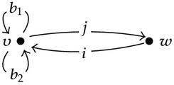
The classification of toric fixed points is given in [49], by identifying the instanton moduli space 𝔐1,k(2) with the Hilbert scheme of points (2) [k]. The fixed points are point-like instantons which are in one-to-one correspondence with Young tableaux λ having |λ | = k boxes. In the more general case of a U(N) gauge theory in the Coulomb branch, one takes N copies of the U(1) theory and the fixed points are classified in terms of N-tuples of Young diagrams , called N-coloured Young diagrams. One can show that the fixed points are isolated.

One can describe the local structure of the instanton moduli space by using the ADHM construction at the fixed points of the action. Following [49], one introduces a two-dimensional T2-module to keep track of the toric action. The operators (B1, B2, I, J) corresponding to a fixed point configuration are elements of the -modules
(4.19)
Then the local structure of the instanton moduli space is described by the complex
(4.20)
which is just a finite-dimensional version of the Atiyah-Hitchin-Singer instanton deformation complex (4.10). The map σ corresponds to infinitesimal (complex) gauge transformations while τ is the linearization of the ADHM constraint μc = 0. In general, the complex (4.20) has three nonvanishing cohomology groups. In our case we can safely assume that H0 and H2 vanish. The only nonvanishing cohomology H1 describes field configurations that obey the linearized ADHM constraint μc = 0 but are not gauge variations. It is thus a local model for the tangent space to the instanton moduli space at each -fixed point. Later on we will compute weights of the toric action on the tangent space modelled on (4.20).
The partition function of the U(1) topologically twisted gauge theory on X = 2 is easily computed. The only nontrivial topological charge is the instanton number k = −∫XFF and therefore the partition function has the form
(4.21)
The expansion parameter can be identified in terms of gauge theory variables q : = e2πiτ with
(4.22)
the complexified gauge coupling, which is related to topological string variables at the attractor point. At a toric fixed point, k is identified as the number of boxes in a partition λ. The Euler classes exactly cancel in the localization formula (3.26), and one is left with the sum over fixed points [50]
(4.23)
By Euler′s formula, one has
(4.24)
where p(N) is the number of partitions λ = (λ1, λ2, …) (ordinary, two-dimensional Young tableaux) of degree |λ | = ∑i  λi = N. The function is related to the Dedekind function. It follows that the U(1) partition function
(4.25)
is the generating function for two-dimensional Young diagrams.
This construction can be easily generalized to the nonabelian case. The fixed points are now N-coloured Young tableaux corresponding to a partition of the instanton number k = (k1, …, kN). The instanton action is again equal to k, where the additional factor of N arising from the sum over colours l = 1, …, N cancels with the normalization of the FF term which carries a factor 1/N (the inverse of the dual Coxeter number of the gauge group G = U(N)). The Euler characteristic of instanton moduli space is now
(4.26)
with The U(N) partition function reduces to N copies of the U(1) partition function
(4.27)
This factorization follows from the fact that after toric localization, the gauge symmetry U(N) → U(1) N is broken to the maximal torus. The Coulomb phase corresponds to well-separated D4-branes, but the topological nature of the gauge theory ensures that the partition function is independent of the Higgs moduli representing the lengths of open strings stretching between D-branes. In the rest of this section, we will extend these constructions to generic toric surfaces X.

4.3. Hirzebruch-Jung Spaces

Our main example will be the most general toric singularity in four dimensions, which defines a class of toric Calabi-Yau (hence open) surfaces known as Hirzebruch-Jung spaces C = C(p, n). They are determined by two relatively prime positive integers p and n with p > n. Consider the quotient singularity 2(p,n), with the generator of the cyclic group Γ(p,n)p acting on (z, w) ∈ 2 as
(4.28)
This orbifold has an Ap,n singularity at the origin of 2. Then C(p, n) is defined to be the minimal resolution of the Ap,n singularity by a chain of exceptional divisors Si1 whose intersection numbers are summarized in the intersection matrix
(4.29)
which is called a generalized Cartan matrix. The divisors thus only intersect transversally with their nearest neighbours in the chain. The self-intersection numbers ei ≥ 2 of the spheres 1 of the blow-up are determined from the continued fraction expansion
(4.30)
Let us consider two particular well-known instances of these spaces.

4.3.1. Local 1

Setting n = 1, the space C(p, 1) can be identified with the total space of the holomorphic line bundle over 1 of degree −p, with = 1 and e1 = p. In this case, S = 1 is the zero section divisor. In the context of topological string theory, such four cycles appear in the “local” Calabi-Yau threefolds X which are regarded as neighbourhoods of a holomorphically embedded rational curve in a compact Calabi-Yau threefold, that is, as the normal bundle 𝒩1. Since 𝒩 is a holomorphic vector bundle of rank two over 1 and the Calabi-Yau condition implies c1(𝒩) = −χ(1) = −2, it follows that X is the total space of a bundle of the form .

4.3.2. Ap−1 ALE Space

The complex surface C = C(p, p − 1) is an example of an asymptotically locally Euclidean (ALE) space. This means that C carries a scalar flat Kähler metric g such that (C, g) is complete, and there exists a compact set K such that . Here pO(4) acts freely on and the metric g approximates the flat Euclidean metric on 4. Such a coordinate system is called a coordinate system at infinity. We regard pU(2) acting on (z, w) ∈ 24 as described above (with n = p − 1), and the complex structure I on C approximates that on 2 = 4. As the resolution of the Klein singularity 2/p, C(p, p − 1) contains a chain of = p − 1 projective lines 1, each with self-intersection number ei = 2. In this case, the intersection matrix C coincides with the Cartan matrix of the Ap−1 Dynkin diagram.

4.4. Instantons on ALE Spaces

We begin by describing in some detail the instanton moduli space in the case of the Ap−1 ALE spaces, for which a rigorous construction is known. U(N) instantons on ALE spaces are given by the ADHM construction. Since the topological gauge theory is invariant under blow-ups of the surface (using blow-up formulas), one can do the instanton computation on the orbifold 2/Γ where Γ = Γ(p,p−1)p. This result is at the heart of the McKay correspondence which provides a one-to-one correspondence between irreducible representations of the orbifold group Γ and tautological bundles over the exceptional divisors of the minimal resolution C = C(p, p − 1).

Since C is noncompact, the instanton moduli space 𝔐C must be defined with respect to connections which have appropriate asymptotic decay at infinity. We will describe this in more generality later on in terms of framed moduli spaces of torsion-free sheaves. These connections correspond to instantons of finite energy and are asymptotic to flat connections with F = 0. In particular, there are solutions which have fractional first Chern class and are related to instantons that asymptote to flat connections with nontrivial holonomy at the boundary of C, which is topologically the Lens space L(p, p − 1) = S3/Γ. The flat connections are classified by homomorphisms ρ : π1(C) → U(N), where π1(C) = Γ≅p. The asymptotic connection at infinity is thus labelled by irreducible representations (k0, k1, …, kp−1) of the orbifold group p, with ∑iki = N, and are given explicitly by
(4.31)
where k = 0,1, …, p − 1.
Starting from the ADHM construction on 2 outlined in Section 4.2., one constructs its Γ-invariant decomposition. Consider the universal scheme 𝒵C × 2 given by the correspondence diagram
image(4.32)
The tautological bundle on C is defined by
(4.33)
Under the action of Γ on 𝒵, transforms in the regular representation and can thus be decomposed into irreducible representations
(4.34)
By the McKay correspondence, the bundles 0 = 𝒪C, 1, …, p−1 form the canonical integral basis of the K-theory group K0(C) constructed in [51].
In this case, we take to be a module on which the regular representation of Γ acts. We also take Γ ⊂ SU(2) so that the determinant representation is trivial as a Γ-module, that is, . The two vector spaces V and W which feature in the ADHM construction have a natural grading under the action of the orbifold group Γ given by
(4.35)
The modification of (4.20) is given by [52]
(4.36)
and the condition that the sequence (4.36) is a complex is equivalent to the (generalized) ADHM equations. After imposing a certain stability condition, this construction realizes the instanton moduli space as a quiver variety 𝔐(V, W).
This construction identifies two distinct types of instanton contributions to the ALE partition function, which we consider in turn. As before, after toric localization the gauge symmetry breaks as U(N) → U(1) N and the U(N) partition function factorizes as
(4.37)
It therefore suffices to focus on the U(1) case in the following.

4.4.1. Regular Instantons

Regular instantons on Ap−1 live in the regular representation k0 = k1 = ⋯ = kp−1 = k of the orbifold group Γ = p. They correspond to D0-branes moving freely on C with p orbifold images away from the orbifold point. For gauge group U(1), the moduli space is given by specifying K = kp points on C up to permutations. Hence the moduli space of regular U(1) instantons on C is isomorphic to the Hilbert scheme C[K]. The generating function for the Euler numbers of the instanton moduli spaces can then be computed explicitly by applying Göttsche′s formula to get
(4.38)
The U(N) partition function is the Nth power of this quantity. Heuristically, we may think of this formula as originating by covering C with p = χ(C) open charts to get p copies of U(N) instantons on 2, each contributing . This can be demonstrated rigorously on any toric surface C by a localization computation [53, 54].

4.4.2. Fractional Instantons

To each irreducible representation (k0, k1, …, kp−1) of the orbifold group p, there corresponds a fractional instanton which is stuck at the orbifold points. It has no moduli (or orbifold images) and can be regarded as a state in which open strings ending on the same D0-brane are projected out by the action of the orbifold group. They carry magnetic fluxes through the 1′s of the minimal resolution, and correspond to self-dual U(1) gauge connections with curvatures
(4.39)
where ui and are the tautological line bundles. The Chern classes c1(i), i = 1, …, p − 1, form a basis of H2(C, ). Fractional instantons can thus be thought of as Dirac monopoles on the two-spheres of the orbifold resolution.
The corresponding intersection numbers are given by
(4.40)
Since C is noncompact, the intersection matrix C is not necessarily unimodular, and the corresponding instanton charges can be fractional. The contribution of fractional instantons to the supersymmetric Yang-Mills action with observables is thus given by
(4.41)
with . Setting u : = (u1, …, up−1) and identifying using the attractor mechanism, we find that the contribution of U(1) fractional instantons to the full partition function is given by a theta-function
(4.42)
on a Riemann surface of genus g = p − 1 and period matrix τC−1.

4.5. Instantons on Local 1

Let us now discuss what is known beyond the ALE case, in the instance that C is the total space of the holomorphic line bundle [55]. In this case an ADHM construction is not available. Nevertheless, much of the construction in the ALE case carries through, and by introducing weighted Sobolev norms, one shows that 𝔐C is a smooth Kähler manifold with torsion-free homology groups which vanish in odd degrees. Let us consider some explicit examples.

The zero section of , considered as a divisor S = 1 of C, produces a line bundle C such that c1() is the generator of H2(C, ) = . It has a unique self-dual connection asymptotic to the trivial connection. Let be the trivial line bundle over C. Set , and let 𝔐() be the moduli space of self-dual connections on which are asymptotic to the trivial connection at infinity. Then dim (𝔐()) = 2p. Since H1(C, ) = 0, using Morse theory one can show that the only nonvanishing homology groups of the instanton moduli space are H0(𝔐(), ) = H2(𝔐(), ) = .

Alternatively, set = , and let 𝔐(k)(), k = 0,1, …, p − 1, be the moduli space of self-dual connections asymptotic to . Then for any p > 2, dim (𝔐(k)()) = 2, while for p = 2 (whereby coincides with the A1 ALE space), one has dim (𝔐(k)()) = 4. In particular, for p = 2 there is a diffeomorphism 𝔐(k)()≅T*1 with H0(𝔐(k)(), ) = H2(𝔐(k)(), ) = , while for p = 4 one has 𝔐(k)()≅B2. Instantons on local 1 will be studied in more generality later on in terms of moduli spaces of framed torsion-free sheaves.

4.6. Wall-Crossing Formulas

In [56] it was suggested that the structure of the instanton partition function on ALE spaces can be extrapolated to give a general result valid for all Hirzebruch-Jung surfaces C = C(p, n). Thus one postulates the form of the U(N) partition function
(4.43)
where
(4.44)
In the ALE case, one has χ(Ap−1) = p and b2(Ap−1) = p − 1. The evidence for this formula is supported by calculations in the reduction to q-deformed two-dimensional Yang-Mills theory [13, 57], which captures the contributions from fractional instantons on the exceptional divisors. It was even conjectured to hold in the case when C is a compact toric surface, at least in the region of moduli space where the instanton charges are large. Though the regular and fractional instantons are always readily constructed exactly as in the ALE case, the issue is whether or not this formula takes into account all of the instanton contributions, and in which regions of moduli space the factorization into U(1) partition functions holds. Later on we will give more precise meanings to these “asymptotic charge regions” in terms of moduli spaces of torsion-free sheaves.
Curiously, the formula (4.43) coincides with the chiral torus partition function of a conformal field theory in two dimensions with central charge c = N  χ(C), that is, of N  χ(C) free bosons, with N  b2(C) of them being compact. The compact degrees of freedom live in a torus determined by the lattice H2(C, ) with the bilinear form C. The appearence of this two-dimensional field theory can be understood in M-theory, wherein the D4-D2-D0 brane quantum mechanics lifts to a (4,0) two-dimensional superconformal field theory on an M5-brane worldvolume [58]. This is reminscent of the recent conjectural relations between four-dimensional superconformal gauge theories and two-dimensional Liouville conformal field theories [59, 60]. When C is an Ap−1 ALE space and the gauge group is SU(N), there is yet another conformal field theoretic interpretation [46, 55, 61, 62]. In this case, the level N affine Lie algebra acts on the cohomology ring of the instanton moduli space, and the partition function (with appropriate local curvature and signature corrections inserted) coincides with the character of the affine Kac-Moody algebra given by
(4.45)
where u = c1(𝒫), n = c2(𝒫) = k + (1/2)  u · Cu, and Ω(n, u) are the degeneracies of BPS states with the specified quantum numbers. Here is the Hilbert space on which the chiral algebra acts, which can be represented in terms of free fermion or boson conformal field theories with extended symmetry generators J0 [61]. The U(1) partition function is also expressed as a character in [61, 62].
Let us now compare the instanton partition function (4.43) with the black hole partition function. Microscopic black hole entropy formulas for BPS bound states of D0-D2-D4 branes in Type IIA supergravity are readily available on compact Calabi-Yau threefolds X [58], in the large volume limit and when contributions from worldsheet instantons are negligible. In this limit we can expand the cycle [C] as in (2.20). Let αi,   i = 1, …, b2(X), be an integral basis of two cocycles for H2(X, ) dual to the four-cycle[Ci] with the intersection numbers
(4.46)
and let Dij be the matrix inverse of . The genus zero topological string amplitude F0 can be expressed as
(4.47)
With 𝒬0 = (1/8π2)∫CFF and , the black hole entropy is given by [58]
(4.48)
We would now like to interpret the gauge theory partition function (4.43) as the corresponding black hole partition function . For this, we expand it as
(4.49)
Then Cardy′s formula gives the black hole entropy as
(4.50)
This expression agrees [56] with the macroscopic supergravity result (4.48) for the Bekenstein-Hawking-Wald entropy in the large 𝒬0 limit. Wall-crossing issues in a similar context are discussed in more detail in [6367].
In parallel to what we did in Section 3.9., in order to explore the pertinent wall-crossing formulas in this instance, we will now consider moduli spaces which parametrize isomorphism classes of the following objects:
  • (a)

    surjections (framings) 𝒪C → 0 of torsion-free sheaves with ch() = (N, d, −k),

  • (b)

    stable torsion-free sheaves on C with ch() = (N, d, k),

  • (c)

    closed subschemes SC of dimension ≤1 with dual curve class [S]  = d and holomorphic Euler characteristic χ(𝒪S) = k.

In contrast to the six-dimensional situation, in four dimensions the connections between these three classes of objects are somewhat more subtle. We will examine each of them in turn and how they compare with the gauge theory results we have thus far obtained.

4.7. Moduli Spaces of Framed Instantons

We begin with Point (a) at the end of Section 4.6. Let C be a smooth, quasiprojective, open, toric surface. We will assume that C admits a projective compactification , that is, is a smooth, compact, projective, toric surface with a smooth divisor (called the “line at infinity”) which is a T2-invariant 1 in , and such that . We will also require that · > 0, in addition to 1. The difference between the counting of framed instantons on the compact toric surface (with boundary condition at “infinity”) and of unframed instantons on the open toric surface C is a universal perturbative contribution, which will be dropped here. Since is compact, these calculations will only capture the contributions from instantons with integer charges on C. We will mention later on how to incorporate the contributions from fractional instantons on C.

Let us fix two numbers N and k, and an integer cohomology class . Let 𝔐N,d,k(C) be the framed moduli space consisting of isomorphism classes [] of torsion-free sheaves on such that
  • (1)

    has the following topological Chern invariants:

    (4.51)

  • (2)

    is locally-free in a neighbourhood of , and there is an isomorphism called the “framing at infinity”.

These topological conditions imply that the moduli space 𝔐N,d,k(C) is nonempty only when
(4.52)
so that d defines a class in the compactly supported cohomology of C. Furthermore, from ch2() = −c2() + (1/2)c1()∧c1(), the last relation in (4.51) can be written as
(4.53)
Framed sheaves yield stable pairs [68], analogous to those described in Section 3.9., after suitable choices of polarization on and stability parameter.
We write . At a given point [] ∈ 𝔐N,d,k(C), the space of reducible connections is , the Zariski tangent space is , and the obstruction space is . The cohomology of the instanton deformation complex is greatly simplified by the fact that in this case [69]
(4.54)
Using (4.54) and the Riemann-Roch theorem, one shows [69] that the moduli space 𝔐N,d,k(C) is a smooth quasiprojective variety of (complex) dimension 2N  k + d2, where d2 : = ∫C  dd, whose tangent space at a point [] is isomorphic to the vector space .

We will now describe a natural torus invariant subspace of the instanton moduli space. The T2-invariance of implies that the pullback of the T2-action on defines an action on 𝔐N,d,k(C). There is also an action of the diagonal maximal torus TN of GL(N, ) on the framing. Altogether we get an action of the complex algebraic torus on 𝔐N,d,k(C) [69]. We are interested in the fixed point set of this torus action.

An isomorphism class [] ∈ 𝔐N,d,k(C) is fixed by the TN-action if and only if it decomposes as
(4.55)
such that is mapped to the lth factor of under the framing isomorphism. Since the double dual is a line bundle which is trivial on , it is equal to for some divisor disjoint from . Via the natural injection , the sheaf l is thus equal to for some ideal sheaf l of a zero-dimensional subscheme also disjoint from . If is also fixed by the T2-action, then so are Dl, l, and Zl.
The supports of the T2-invariant subschemes Zl and Dl can be represented explicitly in terms of the toric geometry of C. Recall that this is described in terms of an underlying toric graph Δ(C) whose vertices are in bijective correspondence with the T2-fixed points in C, and two vertices are joined by an edge e if and only if the corresponding fixed points are connected by a T2-invariant 1. Let V(C) and E(C), respectively, denote the set of vertices and edges of Δ(C). Then since Δ(C) is a chain, one has |E(C)| = |V(C)| − 1. The number of vertices n = |V(C)| is also the number of two-cones in the toric fan of C and it is related to the Euler characteristic χ(C) of the surface as
(4.56)
We denote by pf the T2-invariant point in C corresponding to the vertex fV(C) and by e the T2-invariant line 1 corresponding to the edge eE(C).

Since the zero-cycles Zl are not supported on , they must be contained in the fixed point set V(C) in C. Thus each Zl is a union of subschemes fV(C) supported at the T2-fixed points pfC. If we choose a local coordinate system (x, y) ∈ 2 in a patch Uf around pf, then the T2-invariant ideal of in the coordinate ring [x, y] of Uf2 is generated by the T2-eigenfunctions with nontrivial characters, which are monomials xiyj, and hence corresponds to a Young diagram with boxes (with monomial xiyj placed at (i + 1, j + 1)). The ideal is spanned by monomials outside the Young diagram. Likewise, since the T2-invariant two-cycles Dl are disjoint from the line at infinity, they are supported along the edges e1, eE(C).

It follows that the fixed point set is parameterized by finitely many N-tuples
(4.57)
where
(4.58)
are T2-invariant divisors in C and
(4.59)
is a vector of Young tableaux with boxes. The Young tableaux parametrize the contributions from regular pointlike D0-brane instantons (freely moving inside C). The divisors parametrize the contributions from D2-brane instantons (wrapping Dl with appropriate units of magnetic flux). We will see that these two types of contributions factorize completely. We can write the topological invariants of a generic element (4.57) in in terms of this combinatorial data. Since c1(l) = 0, the constraint d = c1() can be written as
(4.60)
whereas (4.53) becomes
(4.61)
The Young diagram box sum in (4.61) gives the length of the singularity set of the sheaf (4.55).
To make contact with our previous formulas, let us rewrite these constraints in a more explicit parametrization. Define the invertible, symmetric, integer-valued intersection matrix between lines of the toric graph Δ(C) as
(4.62)
Each divisor e is canonically associated to a T2-equivariant holomorphic line bundle e : = 𝒪C(e) whose first Chern class is Poincaré dual to e with
(4.63)
Note that these intersection numbers differ from (4.40), that is, the basis of line bundles e does not coincide with the tautological line bundles i. Using (4.58) we can write with . Then the constraint (4.60) can be expressed as
(4.64)
Combined with (4.61) and using (4.63), this gives
(4.65)
The Vafa-Witten-Nekrasov partition function on the toric surface C is now defined as the -equivariant index
(4.66)
where as before q = e2πiτ with τ the complexified gauge coupling constant and
(4.67)
for a collection of formal variables Qe, eE(C) and a given cohomology class . From the localization formula (3.25), we see that the -equivariant Euler class cancels in (3.26) at the fixed points. This cancellation in the fluctuation determinants is a consequence of (4.54) which implies that the obstruction bundle is trivial, and there is an isomorphism between the tangent and normal bundles over the fixed point set in the instanton moduli space. Because of this cancellation, we see that the contribution from each critical point of the gauge theory is independent of the equivariant parameters ϵi and al. In the sum over critical points, we can replace the sum over k using (4.65) by sums over Young diagrams and over the integers and representing magnetic fluxes through e on D2-branes wrapping the divisors Dl. The sum over may then be saturated using (4.64).
Putting everything together, and using (4.64) and (4.63) to write
(4.68)
the partition function (4.66) thereby becomes
(4.69)
where we have used (4.44). The sums over Young tableaux decouple, and for each vertex fV(C) and each l = 1, …, N, they produce a factor of the Euler function . Then we can bring (4.69) into the final form
(4.70)
where we recall that χ(C) = |V(C)| = n and b2(C) = |E(C)| = n − 1.

This formula differs from (4.43) in that only integral values of the first Chern class are permitted in (4.70). In the case of an Ap−1 singularity, fractional first Chern classes can be incorporated by constructing instead the moduli space of torsion-free sheaves on the orbifold compactification of the hyper-Kähler ALE space C, where [52, 55, 70, 71]. In a neighbourhood of infinity, we can approximate by 2/Γ with the singularity at the origin resolved. More precisely, we obtain the divisor by gluing together the trivial bundle 𝒪C on C with the line bundle on 2/Γ. The latter bundle has a Γ-equivariant structure such that the map is Γ-equivariant. Let us examine some examples which are covered by the analysis above.

4.7.1. Affine Plane

Let C = 2. Then with = [0, z1, z2]≅1 and intersection number · = 1 > 0. Since H2(2, )≅ in this case, the constraint (4.52) implies d = 0. The instanton moduli space 𝔐N,k(2) in this case is a smooth variety of complex dimension 2N  k. Furthermore, n = χ(2) − 2 = 3 − 2 = 1. The partition function (4.66) computed with fixed d = 0 and n = 1 is thus given by
(4.71)
which coincides with the instanton partition function on 2 described in Section 4.2.

4.7.2. Local 1

Let C = Cp, p > 0, be the total space of the holomorphic line bundle of degree −p over 1. Then is the pth Hirzebruch surface. Let and . Then 0 · 0 = −p < 0,    · = p > 0, and 0 · = 0 so that the line 0 does not pass through the “line at infinity”. From the constraint (4.52) and the second Betti number b2(Cp) = 1, it follows that for some m. In this case, the instanton moduli space 𝔐N,m,k(Cp) is a smooth variety of complex dimension 2Nkpm2. The positivity of this dimension is a constraint on the integral classes which ensures that the moduli space is non-empty. One has χ(𝔽p) = 1 + 2 + 1 = 4, and hence n = χ(𝔽p) − 2 = 2. The partition function (4.70) in this case becomes
(4.72)
with u = u1 + ⋯+uN.
Like the ALE spaces, one can work instead with a stack compactification of the total space of the bundle obtained by adding a divisor . The resulting variety is a toric Deligne-Mumford stack whose coarse space is the Hirzebruch surface 𝔽p [72]. With this compactification, one produces framed sheaves with fractional first Chern classes , m, and in this case the partition function takes the form [72]
(4.73)
anticipated by [13, 56], where q = e2πiτ, Q = e2πiv, and is a Jacobi elliptic function.

On these spaces, one also has a version of the Hitchin-Kobayashi correspondence which makes contact with the realization of instantons as self-dual connections. Namely, SU(N)-instantons on Cp are in one-to-one correspondence with holomorphic bundles of rank N on Cp with c1() = 0 together with a framing at infinity [73]. When p = 2, these spaces coincide with the A1 ALE space.

4.7.3. Compact Surfaces

We will now examine situations under which the formula (4.70) holds in the case of compact surfaces, providing rigorous justification for some of the conjectural formulas of [56]. Let C be a compact, smooth, projective toric surface. Let c be a generic point in C which is disjoint from the torus invariant lines e, eE(C) of C. Let 𝔐N,d,k(C, c) be the moduli space of isomorphism classes [] of torsion-free coherent sheaves on C with topological Chern invariants as in (4.51), together with a “framing” at the point c. When is locally free, this framing means a choice of basis for the fibre space . When is not locally free, the framing is defined with respect to a locally free resolution → 0.

Let be the blow-up of C at c. Then is also a compact, smooth, projective toric surface. We will suppose that the exceptional divisor has positive self-intersection . Let be the moduli space of isomorphism classes of torsion-free sheaves on which are framed on the line as above. The blow-up map σ determines mutually inverse sheaf morphisms and , and hence an explicit isomorphism
(4.74)
It follows from above that the moduli space 𝔐N,d,k(C, c) is thus a smooth variety of complex dimension 2N  k + d2, where d2 : = ∫C  dd. Using the isomorphism (4.74), the instanton partition function on C can be computed from the blow-up formula
(4.75)
where the right-hand side is given by the formula (4.70).
As an explicit example, consider the complex projective plane C = 2. Let z be a generic point on 2 disjoint from the line = [0, z1, z2]. Then the instanton moduli space 𝔐N,d,k(2, z) is a smooth variety of complex dimension 2N  k + d2, where d. Let be the blowup of 2 at z with exceptional divisor . Then there are maximal two cones and edge in the toric graph . Since · = 1 in this case, the partition function (4.75) gives the U(N) formula
(4.76)
with u = u1 + ⋯+uN. For N = 1 this agrees with the U(1) gauge theory partition function on 2 derived in [54, Section 5.1].

4.8. Stability

Next we address Point (b) at the end of Section 4.6. If one wishes to relax the requirement of framing, then one must carefully analyse stability issues in order to obtain well-defined instanton moduli spaces. Let C be a smooth, quasiprojective toric surface. Again we fix invariants N, k, and . Let 𝔐N,d,k(C) be the unframed moduli space consisting of isomorphism classes [] of semistable torsion-free coherent sheaves on C such that has topological Chern invariants
(4.77)
The notion of “semistability” considers sheaves with fixed Hilbert polynomial. In this case, a general result of Maruyama [74, 75] constructs the algebraic scheme 𝔐N,d,k(C) and shows that it is projective. In particular, it admits a -equivariant embedding into a smooth variety. In the case that C is a polarized surface, that is, it admits a smooth distribution in its tangent bundle TC which is integrable and Lagrangian (in an appropriate sense), we can formulate the notion of semistability in terms of the more familiar slope semistability following [76]. Let be a fixed ample line bundle on C. For a coherent torsion-free sheaf on C, define the polynomial
(4.78)
for n0. Then is said to be -semistable if
(4.79)
for all n ≫ 0 whenever is a coherent subsheaf of . In this case, Gieseker [76] constructs 𝔐N,d,k(C) as a projective Quot scheme. The slope of is the rational number
(4.80)
where the degree of is defined using the polarization as
(4.81)
An application of the Riemann-Roch theorem shows [76]
(4.82)
It follows that ρ(n) ≥ ρ(n) for n ≫ 0 if and only if μ() ≥ μ(), and hence -semistability is equivalent to the usual quasi-BPS instanton equations in this case. In physics applications, one is interested in instances where C is a Kähler surface. In this case one can use the Kähler polarization and take c1() to be the Kähler two-form k0 in (4.32).

The following result computes the expected dimension of the instanton moduli space in this case.

Lemma 4.1. The virtual dimension of 𝔐N,d,k(C) equals 2N  k + d2 − (N2 − 1)  χ(𝒪C), where d2 : = ∫Cdd and χ(𝒪C) is the holomorphic Euler characteristic of C.

Proof. As discussed in Section 3.5., the dimension of the virtual tangent space to the instanton moduli space at a point [] ∈ 𝔐N,d,k(C) in obstruction theory is the difference of Euler characteristics . The latter quantity may be computed for locally free by using the Hirzebruch-Riemann-Roch theorem to write

(4.83)
Let ν be the generator of H4(C, )≅ which is Poincaré dual to a point in C. Then using (4.77) one computes the Chern character
(4.84)
The Todd characteristic class of the tangent bundle of C is given in terms of Chern classes of TC as
(4.85)
We may thus write (4.83) as
(4.86)
From the Hirzebruch-Riemann-Roch formula and ch(𝒪C) = 1, one has
(4.87)
and the result follows when is a bundle. When is not locally free, we use a locally free resolution → 0 along with additivity of the Chern character.

This result shows that the expected dimension of the instanton moduli space for N = 1 coincides with the dimension of the framed moduli space 𝔐1,d,k(C) of Section 4.7. Indeed, torsion-free sheaves of rank one are always stable in the sense explained above. Since any torsion-free sheaf decomposes as the product = of an ideal sheaf of a zero-dimensional subscheme and a line bundle, the moduli space factorizes into a product
(4.88)
where 𝔐1,0,K(C)≅C[K] is the Hilbert scheme of K points on C which is a smooth variety of dimension 2K, and the (zero-dimensional) Picard group parameterizes fractional instantons. The factorization of the U(1) gauge theory partition function into contributions from regular and fractional instantons then follows from the multiplicativity of the Euler class under tensor product of (tangent) bundles. For compact toric surfaces C, it is given by the formula (4.70) with N = 1. In the case of Hirzebruch-Jung surfaces, the contributions of fractional charges in this case are shown in [54] to arise from the noncompact prime divisors of C via linear equivalences. It amounts to identifying the generators c1(i) of the Kähler cone in CH1(C) ⊗ with the duals to the exceptional divisors Di which generate the Mori cone in . For the ALE spaces, the moduli space coincides with the quiver variety of the ADHM construction (with suitable stability conditions) [77].

The situation for higher rank N > 1 is much more complicated. In this case, slope-stability does not seem to properly account for walls of marginal stability extending to infinity which describe wall-crossing behaviour of the partition functions counting D4-D2-D0 brane bound states on Calabi-Yau manifolds X with h1,1(X) > 1 [64]. As discussed in Section 3.9., the physical theory is described by moduli spaces of stable objects in the derived category Db(coh(X)), as the observed D-brane decays are impossible in the abelian category coh(X) of coherent sheaves on X.

4.9. Perpendicular Partition Functions and Universal Sheaves

Finally, we come to the last Point (c) at the end of Section 4.6. For U(1) gauge theory, this relationship is analysed in detail in [54]. In this case a four-dimensional analog of the topological vertex formalism can be developed. On the gauge theory side, the vertex contributions should be computed by a version of the perpendicular partition function of Section 3.8., that is, the generating function for instantons on C = 2 with fixed asymptotics such that , while the edge contributions should be read off from the character of the corresponding universal sheaf. In the remainder of this section, we will describe in detail the instanton moduli space with boundary conditions specified by integers m1, and m2, and show that the fixed point loci of the induced -action are enumerated by two-dimensional Young diagrams with asymptotics m1, and  m2. This gives the four-dimensional version of the gauge theory gluing rules of Section 3.8. and also a first principle derivation of the empirical vertex rules of [54, Section 4.3].

4.9.1. Instanton Moduli Spaces on 𝔽0

We will first describe how to generate instantons with nontrivial first Chern class using our previous formalism. For this, rather than working with the projective plane , it is more convenient to work with the “two-point compactification” of C = 2 given by a product of two projective lines , where the labels will be used to keep track of each of the two factors. This variety can be identified as the zeroth Hirzebruch surface , that is, the projective compactification of the trivial line bundle , which is again a toric surface. For (tz, tw) ∈ T2, the toric action is described by the automorphism of 𝔽0 defined by
(4.89)
Let pz :  and pw :  be the canonical projections, and and iw :  the natural inclusions. There are now two independent distinguished lines at infinity fixed by this T2 action, given by the pushforwards and , for which the respective factors of the action of T2 = * × * reduce to the standard *-action on z, w1. These two divisors have intersection products z · z = w · w = 0 and z · w = 1, and the canonical divisor is . They generate the Picard group of 𝔽0, and hence induce a bigrading on line bundles over 𝔽0. For mz, mw, we write
(4.90)
By Künneth′s theorem, the nontrivial cohomology groups of 𝔽0 are given by
(4.91)
where and .

Let be the moduli space of isomorphism classes [] of torsion-free sheaves on 𝔽0 with topological Chern invariants as in (4.51), where d = mzξz + mwξw, and nontrivial framings along the two independent “directions at infinity” are prescribed by two fixed isomorphisms and , where W is a fixed N-dimensional complex vector space. We will say that such a sheaf is “trivialized at infinity” if it is equipped with two isomorphisms and . The moduli space of trivialized sheaves is denoted 𝔐N,k(𝔽0): = 𝔐N;(0,0);k(𝔽0). These moduli spaces carry an obvious induced action of the torus , and the following formal arguments show that the instanton counting in these moduli spaces is the same as before.

Proposition 4.2. There is a natural -equivariant birational equivalence between the moduli spaces

(4.92)

Proof. Represent 𝔽0 as a divisor in 2 × 1 via the embedding , [z0, z1]↦[z0, z1, z1]. Let be the surface obtained as the blowup p of a pair of points on the line at infinity 2 (see Section 4.7.). Note that is disjoint from the image of the line z. Then there is a correspondence diagram

image(4.93)
where q is the blowup of the intersection point z · w on . The corresponding Fourier-Mukai functors q*p* and p*q* determine equivalences on the categories of coherent sheaves over 2 and 𝔽0, and hence induce mutually inverse rational maps between the corresponding sets of isomorphism classes of trivially framed torsion-free sheaves.

Proposition 4.3. For each fixed (mz, mw) ∈ 2, there is a natural -equivariant bijection between the moduli spaces

(4.94)
where
(4.95)

Proof. Given [] ∈ 𝔐N,k(𝔽0), define

(4.96)
By (4.51) (with d = 0), one has
(4.97)
and using multiplicativity of the Chern character we compute
(4.98)
This therefore gives a map []↦[(mz, mw)] on . An identical calculation shows that the map is its inverse. These maps clearly induce bijections between (mz, mw)-framings and trivializations at infinity.

Proposition 4.2 shows that an instanton gauge bundle with trivial asymptotics on 𝔽0 can again be regarded as an element [] ∈ 𝔐N,k(2). For fixed mz, mw, Proposition 4.3 shows that the counting of torsion-free sheaves in the moduli spaces 𝔐N,k(𝔽0) and coincides. In other words, the number of instantons with fixed nontrivial asymptotics matches the Young tableau count, as the number of sheaves (4.96) is independent of the integers mz, mw. Proposition 4.3 also reproduces the formula [54, Section 4.2.2] for the renormalized volume of Young tableaux (reproduced above for N = 1) as the induced shift in instanton charge in (4.95) of the sheaves (4.96).

The bijection of Proposition 4.2 is not necessarily a diffeomorphism. In fact, we have not yet shown that 𝔐N,k(𝔽0) is a smooth variety. Naively, one may try to argue this by using the formalism of [69], as our sheaves are trivialized on the divisor = z + w which has positive self-intersection · = 2, and 𝔽02. However, this divisor is not irreducible; in particular, it is not a 1. Note that formally applying the arguments which led to (4.72) in the limit p = 0 would produce the partition function
(4.99)
as the Hirzebruch surface has n = χ(𝔽0) − 2 = 2. Although the generating function (4.99) is “doubled”, the instanton counting problems on 𝔽0 and on 2 are nevertheless identical. A rigorous derivation of the formula (4.99) using the techniques of Section 4.7. follows once we establish that the equivalence of Proposition 4.2 is an isomorphism of underlying smooth varieties. Recall from Section 4.7. that the complex dimension of the instanton moduli space 𝔐N,k(2) is 2N  k.

Proposition 4.4. The moduli space 𝔐N,k(𝔽0) is a smooth quasiprojective variety of complex dimension 2N  k.

Proof. As usual, the trivialization condition at infinity guarantees Gieseker semistability and hence quasi-projectivity, as discussed in Section 4.8. Using the divisor = z + w of 𝔽0, one constructs the framed moduli space 𝔐N,k(𝔽0) as in [68] with tangent spaces and obstruction spaces given by . By reference [78, Section 5], one has

(4.100)
and hence 𝔐N,k(𝔽0) is smooth. The dimension of the tangent spaces is thus equal to minus the Euler characteristic −χ(, (−1, −1)), which for locally free may be calculated by using the Hirzebruch-Riemann-Roch theorem to write
(4.101)
Using (4.97) and (4.98), one computes the Chern character
(4.102)
The Todd characteristic class and holomorphic Euler characteristic are given by (4.85) and (4.87) with C = 𝔽0, and we may thus write (4.101) as
(4.103)
One has since b2(𝔽0) = 2 = h1,1(𝔽0). Since ξz, ξwH2(𝔽0, ) are the Poincaré duals of [z], [w] ∈ H2(𝔽0, ), with z, w1 and z · z = w · w = 0, the remaining integral in (4.103) may be computed as
(4.104)
where in the last step we used the fact that the holomorphic tangent bundle of 1 can be identified with . Putting everything together, we find
(4.105)
and the result follows when is a bundle. If is not locally free, then we simply consider a locally free resolution → 0 and use additivity of the Chern characteristic class.

In a similar vein, the equivalence established in Proposition 4.3 as it stands is only a bijective correspondence. The moduli space for nontrivial asymptotics is an example of the moduli spaces of “decorated sheaves” described in [20, Section 4.B], with the (mz, mw)-framed sheaves on 𝔽0 providing examples of semistable framed modules. The moduli space is thus a projective scheme with a universal family, that is, it is fine, and so possesses a universal sheaf. We will now argue that the moduli spaces are smooth and diffeomorphic to one another for all mz, mw. Then the computations of Section 4.7. can be repeated by integrating over using (4.95) and Göttsche′s formula to get the desired perpendicular partition function
(4.106)
For N = 1, this yields a rigorous derivation of the vertex rules of [54].

Let be the moduli space of isomorphism classes of pairs , where is an (mz, mw)-framed torsion-free sheaf on 𝔽0 and is the surjective morphism induced by the framing. Consider the family of pairs consisting of a coherent sheaf on 𝔽0 together with a homomorphism for some r. These pairs define objects of an abelian category cohf(𝔽0) with the obvious morphisms between pairs induced by morphisms of coherent sheaves. Any (mz, mw)-framed torsion-free sheaf on 𝔽0 clearly defines an object of cohf(𝔽0), with r = N and ch() = ch().

Given the abelian category cohf(𝔽0), one can derive functors, and hence compute sheaf cohomology in cohf(𝔽0). We denote the corresponding Ext-functors by . Then is the obstruction space for at , while is the tangent space to at . Generally, for any two objects of cohf(𝔽0), the group can be computed in a purely algebraic way in terms of equivalence classes of extensions
image(4.107)

This definition of is equivalent to the usual definition in terms of a twisted Dolbeault complex, and in particular it gives the deformation theory of the moduli space . Furthermore, there is a spectral sequence connecting it to the ordinary Ext-groups .

The line bundle is a projective -module and is therefore flat, whence the tensor product map defined by (4.96) preserves exact sequences such as (4.107). It follows that the tangent spaces are the same for all mz, mw. Thus by Proposition 4.4, the moduli spaces are all smooth and diffeomorphic to one another. This is consistent with the fact that stability (either slope stability of torsion-free sheaves [76] or stability of framed modules [20, Section 4.B]) is preserved by twisting with the line bundles .

4.9.2. Universal Sheaves

We now construct the universal sheaf for the standard framing on 𝔽0, and compute its -equivariant character. Since the moduli space 𝔐N,k(𝔽0) is fine [68], there exists a universal sheaf 𝔈𝔽0 × 𝔐N,k(𝔽0), that is, a torsion-free sheaf 𝔈 such that for every point [] ∈ 𝔐N,k(𝔽0), unique up to tensor product with a (unique) line bundle. There are two natural vector bundles over 𝔐N,k(𝔽0) associated to a universal sheaf 𝔈. Firstly, there is the framing bundle of rank N given by the fibre at infinity. Secondly, there is the bundle V of “Dirac zero modes”, whose fibre at a given locally free sheaf [] ∈ 𝔐N,k(𝔽0) restricted to 42𝔽0 is the space of L2-solutions to the Dirac equation on 4 in the background of the fundamental representation of the instanton gauge field corresponding to . It is constructed explicitly as follows. Let π1 and π2 be the canonical projections of 𝔽0 × 𝔐N,k(𝔽0) onto the first and second factors, respectively. Then the Dirac bundle is
(4.108)
where R1π2* is the first right derived functor of the pushforward functor π2*. Its fibre over a point [] ∈ 𝔐N,k(𝔽0) is the vector space H1(𝔽0, (−1, −1)).

Proposition 4.5. The Dirac bundle V is a vector bundle of rank k over 𝔐N,k(𝔽0).

Proof. By reference [78, Section 5], one has

(4.109)
and hence V is a vector bundle of rank equal to −χ((−1, −1)). For locally free, the Hirzebruch-Riemann-Roch theorem, together with (4.98), (4.85) with C = 𝔽0, (4.104), and gives
(4.110)
Again, the statement for generic torsion-free sheaves [] ∈ 𝔐N,k(𝔽0) follows by considering a locally free resolution → 0.

By definition, (4.89) and the construction of Section 4.7., the -equivariant characters of the framing and Dirac bundles regarded as -modules, at a fixed point in labelled by an N-coloured Young tableau , are given by
(4.111)
where . Let us now describe how the ADHM construction is modified in this case. This has been worked out in [78, Section 5]. The linear algebraic data is formally the same as for the analysis of framed instantons on 2 [49], defined by linear operators
(4.112)
Then any framed torsion-free sheaf [] ∈ 𝔐N,k(𝔽0) can be represented as the middle cohomology group of the complex
(4.113)
which is exact at the first and last terms, where
(4.114)
The virtual -equivariant bundle defined by the cohomology of the complex (4.113) gives a representative of the isomorphism class of the universal sheaf 𝔈 in the -equivariant K-theory group as
(4.115)
where
(4.116)
are -equivariant bundles over 𝔽0 which, after tensoring with a line bundle of degree one, restrict to the usual positive/negative chirality spinor bundles over 42𝔽0. In the topologically twisted gauge theory, fermion fields become differential forms and these bundles are identified with the bundles of even/odd holomorphic forms over 𝔽0 [79]. By (4.89), the holomorphic line bundles (4.90) have -equivariant characters
(4.117)
and consequently,
(4.118)
Using (4.111) and (4.118), we may thus compute the character of the universal sheaf (4.115) at a fixed point in the instanton moduli space as
(4.119)
which coincides with the standard expression for instantons on 4 [80].
For completeness, let us record here the -equivariant Chern character of the tangent bundle T𝔐N,k(𝔽0) over the instanton moduli space at the torus fixed points. As the only nonvanishing cohomology group of (4.20) is a model of the tangent space, it can be computed as the equivariant index of this complex. For this, let us recall some combinatorial definitions. Let λ be a Young diagram. Define the arm and leg lengths of a box (i, j) ∈ λ, respectively, by
(4.120)
where ϱi is the length of the ith column of λ and is the length of the jth row of λ. At a fixed point , the character can then be expressed after some algebra in terms of the characters of the representation as
(4.121)
Again this coincides with the standard result [50, 80, 81]. As in [82], after toric localization one has
(4.122)
at the -fixed points , up to a universal perturbative contribution (the character of WW*). This expression formally generalizes to generic toric surfaces [83] and is used to construct vertex gluing rules below. From the top Chern class, one can also straightforwardly extract the equivariant Euler classes
(4.123)
where
(4.124)

4.9.3. Framed Modules on 𝔽0 from Dirac Modules on 1

For the case of nontrivial (mz, mw)-framings, let
(4.125)
be the isomorphism induced by the map , and let 𝔈 be a universal sheaf on 𝔽0 × 𝔐N,k(𝔽0). Then the torsion-free sheaf
(4.126)
is a universal sheaf on . The equivariant character of 𝔈(mz, mw) at the fixed points of the toric action modifies the decompositions (4.111) to allow for “propagators” which appear along the edges 1 of the toric diagram Δ(C) of a generic toric surface C. These modifications of the -equivariant character of the universal sheaf corresponding to the instanton sheaves (4.96) are determined via shifts by the *-equivariant character of modules of solutions to the Dirac equation on 1. We will now describe these modules explicitly. As we have seen, the bundle of degree m over the Riemann sphere 1 is the crucial ingredient in generating instantons with nontrivial framings. After choosing a hermitean metric on the fibres of , it is the holomorphic line bundle underlying the standard Dirac monopole line bundle of topological charge m. The form of the Dirac operator in the background of the corresponding monopole gauge potential is well known and can be conveniently described in the following way [32].
Given homogeneous coordinates [z0, z1] on 1, let y = z1/z0 denote stereographic coordinates on the northern hemisphere. Then the twisted Dirac operator in the monopole background of magnetic charge m is given by
(4.127)
where
(4.128)
These operators act on sections of the chiral/antichiral spinor line bundles associated to the twisted holomorphic spinor bundles . We are interested in the subspaces of zero modes
(4.129)
The action of t* is implemented by the automorphism Ft of 1 defined by
(4.130)
The irreducible representations of * are labelled by their weights i and are defined by zt · z = ti  z for t* and z. The corresponding *-eigenspace decomposition of the modules (4.129) can be described for all m as follows.

Theorem 4.6. The isotopical decompositions of the spinor modules over 1, as *-modules, are given by

(4.131)

Proof. The solutions of the Dirac equation are given by L2-solutions of the differential equations

(4.132)
for the spinors . The line bundle has holomorphic transition function ym transforming sections from the northern hemisphere to the southern hemisphere of 1, which after unitary reduction to a hermitean line bundle becomes . By using these transition functions, it is easy to see that the only solutions of the equations (4.132) which are regular on both the northern and southern hemispheres are of the form
(4.133)
with constant coefficients . The result now follows from (4.130).

We can use Theorem 4.6 to compute the *-equivariant characters of the spinor modules (4.129). One finds
(4.134)
for m > 0, while
(4.135)
for m < 0. In the nonequivariant limit t → 1, the characters (4.134) and (4.135) reproduce the known index of the Dirac operator, , in the monopole background. These characters shift the character (4.119). For example, with mz, mw > 0 and N = 1, one has
(4.136)
This completes the derivation of the gluing rules of [54, Section 4.3].

5. D2-Brane Gauge Theory and Gromov-Witten Invariants

In this final section, we study the reduction of the four-dimensional gauge theories of Section 4 on local curves and examine in detail the example of local 1 which has been extensively described from the point of view of Vafa-Witten theory. We begin with a somewhat heuristic description of how these two-dimensional supersymmetric gauge theories are induced. Then we proceed to a more formal topological field theory formalism which systematically computes topological string amplitudes and Gromov-Witten invariants. Finally, we briefly address wall-crossing issues once again from a physical standpoint.

5.1. q-Deformed Two-Dimensional Yang-Mills Theory

One of the simplest classes of examples are the noncompact local Calabi-Yau threefolds which are fibred over curves. If ΣgX is a holomorphically embedded curve of genus g in a Calabi-Yau threefold, then the holomorphic tangent bundle restricts to Σg as , where the normal bundle is a holomorphic bundle of rank two over Σg. By the Calabi-Yau condition c1(X) = 0, one has . Thus in a neighbourhood of Σg, the manifold X looks like the total space of a holomorphic bundle 𝒩Σg of rank two with c1(𝒩) = 2g − 2. Hence we consider the total space of the bundle
(5.1)
over Σg. Since is a holomorphic line bundle over Σg of degree p, one has
(5.2)
as required. For genus g = 0, this is just the example of local 1 which was introduced in Section 4.3.
In our applications to black hole microstate counting, we count bound states of D4-D2-D0 branes in Xp with N D4-branes wrapping the four-cycle Cp which is the total space of the line bundle , together with D2-branes wrapping the base Riemann surface Σg (embedded in C and Xp as the zero section). One can then localize the path integral of the 𝒩 = 4 topological gauge theory on Cp to the *-invariant modes along the fibre of . The result is an effective U(N) gauge theory on Σg whose action is given by [84]
(5.3)
where ϑ = gs  ϕ2/2π and the last term is a mass deformation which originates in four dimensions due to the nontriviality of the bundle [85]. The scalar field Φ is given by the holonomy of the four-dimensional gauge connection at infinity
(5.4)
where zΣg and .
The action (5.3) is just the BF-theory representation of two-dimensional Yang-Mills theory, with the usual F2-term coming from performing the gaussian integral over Φ in the functional integral. If Φ were arbitrary, then we could use diagonalization techniques to reduce the partition function to the usual heat kernel expansion of two-dimensional Yang-Mills theory. However, the identification of Φ as a holonomy means that it should be treated as a periodic field, and the change from a Lie algebra-valued variable to a group-like variable affects the Jacobian of the path integral measure that arises from diagonalization. This modifies the usual Migdal expansion of two-dimensional gauge theory to give the partition function
(5.5)
where as before and Q = eiϑ. The sum runs over unitary irreducible representations R = (R1, …, RN) of the gauge group U(N) with weights Ri, first and second Casimir invariants C1(R) = ∑iRi and and quantum dimension
(5.6)
where the q-number is defined by
(5.7)
with [n] q = n + O(q − 1) for q → 1. This reduced two-dimensional gauge theory is a q-deformation of ordinary Yang-Mills theory.

5.2. Topological Field Theory

We will now give a more precise definition of this gauge theory using techniques of two-dimensional topological field theory. This formalism can then be used to compute topological string amplitudes. The idea is that the cutting and pasting of base Riemann surfaces is equivalent to the cutting and pasting of the corresponding local Calabi-Yau threefolds, by either adding or cancelling off D-branes corresponding to the boundaries in the topological vertex formalism [84, 86]. The operations of gluing manifolds satisfy all axioms of a two-dimensional topological field theory. By computing the open string topological A-model amplitudes on a few Calabi-Yau manifolds, we then get all others by gluing. In the following we focus on the genus zero case Σ0 = 1 for simplicity and illustrative purposes.

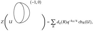
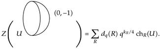
When the base of the fibration is the sphere, we will only need the basic Calabi-Yau cap amplitude corresponding to a disk D, represented symbolically as
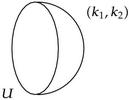
image

where the levels k1 = e(1) and k2 = e(2) label the degrees in H2(D, D) of a pair of line bundles 12D, and the unitary matrix U labels the holonomy of a gauge connection on DS1. Under concatenation the levels add. The basic cap amplitude is defined by

image

where as before, the sum over R runs through the space of symmetric functions (Young tableaux), that is, irreducible representations of SU(), and chR(U) is the character of the holonomy U in the representation R. The quantity
(5.8)
is the quantum dimension of the symmetric group representation corresponding to the Young diagram of R, and
(5.9)
The quantity
(5.10)
is the topological vertex amplitude for the A-model topological string theory with a single stack of D-branes on the noncompact Calabi-Yau threefold X = 3. Similarly, define the cap amplitude

image

For the gluing rules, we sew two open Riemann surfaces ΣL and ΣR together along their common boundary to get the Riemann surface ΣLR. For this, the orientations of the corresponding boundary circles must be opposite. Reversing the orientation acts on the boundary holonomy as UU−1, and hence the gluing rules read
(5.11)
where dU is the bi-invariant Haar measure and the integrals can be evaluated explicitly by using the orthogonality relations for characters
(5.12)
We will also need the Calabi-Yau trinion (or “pants”) amplitudes

image

Let us point out two particularly noteworthy aspects of this construction thus far. Firstly, the construction defines a functor of tensor categories
(5.13)
where Rep is the representation category of SU() and is the geometric tensor category defined as follows. The objects of are compact oriented one-manifold Y, that is, disjoint unions of oriented circles. A morphism Y1Y2 between two objects of is a triple (W, Y1, Y2), where W is an oriented cobordism between Y1 and Y2, that is, a smooth oriented two-manifold with boundary W = Y1 ∐ (−Y2), and the complex line bundles 1, 2 over W are trivialized on W. This is analogous to the Baum-Douglas description of D-branes in K-homology [87]. There is a natural notion of equivalence provided by boundary preserving, oriented diffeomorphisms f : WW with , i = 1,2. Composition of morphisms is given by concatenation of cobordism and gluing of bundles along the concatenation using the trivializations. For a connected cobordism W, we can label the isomorphism classes of a pair of line bundles (1, 2) by the levels (k1, k2), where ki = e(i) ∈ H2(W, W). Under concatenation, these levels add.
Secondly, the *-action on 1 lifts to an action of the torus T = (*) 2 on Xp, via the natural scaling action on the fibres. The Gromov-Witten invariants in this case are defined via the virtual localization formula as a residue integral over the T-fixed point locus, along the lines explained in Section 3.5. A stable map to Xp which is T-invariant factors through the zero section. It follows that there is a natural isomorphism of moduli spaces 𝔐g(Xp, β) T = 𝔐g(1, β), with β = d, and consequently
(5.14)
This equality of virtual fundamental cycles implies that the invariants constructed by integrating over each moduli space coincide. It means that topological string theory on Xp is equivalent to a field theory on 1, which is just the reduction we argued in Section 5.1. In this case the Gromov-Witten invariants of Xp correspond to degree d Hurwitz numbers of 1.

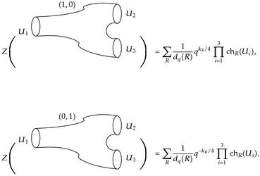
Returning to our computations, we get the annulus (or tube) amplitude by contracting the cap and trinion amplitudes to get
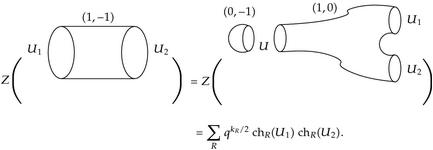
image

Finally, we compute the amplitude of the fibration Xp1 by using (5.14) and the gluing rules. In order to get the appropriate bundle degrees (p − 2, −p), we glue p tubes between two caps to get
image(5.15)

For p = 1, the threefold is the resolved conifold, and this formula is a q-deformation of the classical Hurwitz formula counting unramified covers of the Riemann sphere 1.

In fact, the quantity dq(R) is analogously the N limit of the quantum dimension dim q(R) of the U(N) representation with the same Young tableau. This follows by Schur-Weyl reciprocity which writes SU(N) representations in terms of representations of the symmetric group SN. Let R be a representation corresponding to a Young diagram λ with row lengths λi, i = 1, …, d(λ), where λ1λ2 ≥ ⋯, and d(λ) is the number of rows in λ. Set μ = qN, and define another q-number by
(5.16)
Then the quantum dimension of R can be written as
(5.17)
This is a Laurent polynomial in μ±1/2 whose coefficients are rational functions of q±1/2. The leading power of μ is |λ|/2, and the coefficient of this power is the rational function of q±1/2 given by
(5.18)
As before, this is just the topological vertex amplitude CR,,(q). The limit q → 1 gives the ordinary dimension of the representation R.
Generalizing the generating function (5.15) thereby gives
(5.19)
where now the sum runs over irreducible representations R of U(N) and C2(R) = kR + N(R) is the second Casimir invariant of R. By the attractor mechanism, the Kähler modulus of 1 is given by t = (N/2)  (p − 2)  gs. In the limit q → 1, this two-dimensional field theory coincides with ordinary Yang-Mills theory on the sphere 1. Note that this is a weak-coupling limit gs → 0, with and A the area of 1. Using similar constructions as above, it is possible to formulate this gauge theory directly as a two-dimensional topological field theory, without any reference to the extrinsic bundle structure of the local threefold Xp. Explicit computations of the corresponding Gromov-Witten invariants of Xp can be found in [911].

5.3. Wall-Crossing Formulas

Finally, let us briefly comment on the relationship to black hole entropy counting. Reinstating the ϑ-angle as in (5.5), the attractor mechanism fixes the Kähler modulus of Σ0 = 1 as
(5.20)
The large N limit of the partition function (5.5) should possess this modulus. The modulus squared structure anticipated by the OSV relation (2.25) is given in this limit by [84]
(5.21)
where the sum over r runs through U(1) charges in the local decomposition U(N) ~ U(1) × SU(N) of the gauge group, the second sum runs through pairs of irreducible SU(N) representations R1, R2, and is the perturbative topological string amplitude on Xp with two stacks of D-branes in the fibre. The conjugate amplitude is . Thus in this case the OSV relation (2.25) is modified to the symbolic form
(5.22)
where the first sum runs over Ramond-Ramond fluxes r through the base Riemann surface Σg while the second sum is over fibre D-branes which carry additional moduli measuring their distances from the base Σg along the noncompact fibre directions.

Further analysis of the relationships with 𝒩 = 4 Yang-Mills theory on Cp is studied in [9, 10, 12, 13, 57], where it is observed that the instanton expansions of the two-dimensional and four-dimensional gauge theory partition functions differ by perturbative contributions. These extra factors arise from the noncompactness of the surface Cp. When Cp is the resolution of an Ap,n singularity, its boundary is the three-dimensional Lens space L(p, n) = S3(p,n). The perturbative factors can then be identified as the partition function of Chern-Simons gauge theory on the boundary and arise as a consequence of the fact that the two-dimensional gauge theory implicitly integrates over all boundary conditions. Once these boundary contributions are stripped, the enumeration of instantons in the two-dimensional and four-dimensional gauge theories coincide [13].

Acknowledgments

It is a pleasure to thank M. Cirafici, E. Gasparim, A.-K. Kashani-Poor, A. Maciocia, and A. Sinkovics for enjoyable discussions and collaborations on some of the results presented here. This work was supported in part by Grant ST/G000514/1 “String Theory Scotland” from the UK Science and Technology Facilities Council.

      The full text of this article hosted at iucr.org is unavailable due to technical difficulties.