A heteroscedastic linear regression model is developed from plausible assumptions that describe the time evolution of performance metrics for equipment. The inherited motivation for the related weighted least squares analysis of the model is an essential and attractive selling point to engineers with interest in equipment surveillance methodologies. A simple test for the significance of the heteroscedasticity suggested by a data set is derived and a simulation study is used to evaluate the power of the test and compare it with several other applicable tests that were designed under different contexts. Tolerance intervals within the context of the model are derived, thus generalizing well-known tolerance intervals for ordinary least squares regression. Use of the model and its associated analyses is illustrated with an aerospace application where hundreds of electronic components are continuously monitored by an automated system that flags components that are suspected of unusual degradation patterns.

1. Introduction

1.1. Background

The model and analyses developed in this paper address a problem encountered when analyzing data from service life tests of aerospace hardware packages. Data for as many as 700 performance metrics per part type are automatically stored during surveillance testing and subsequently input into a software program where, up to this point, an ordinary least squares line based on normal-theory has been routinely fit to the data using time-in-service as the explanatory variable. The software program also outputs tolerance intervals based on the ordinary least squares analysis. Engineers monitoring this process are alerted only to those cases where observations in the scatter plot fall outside the tolerance intervals or the tolerance interval crosses a given limit within some specified future time interval (e.g., 60 months). In cases where the alert suggests an increasing accelerated degradation, a proactive corrective action (e.g., part replacement) may be initiated. In cases where the alert suggests less than expected degradation, a cursory investigation to determine if the part is being utilized properly is initiated. Tolerance intervals are often similarly used for monitoring environmental applications [1].

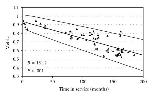
Compared to having engineers individually examine the data from all the combinations of metrics and part types, the automated monitoring and flagging process is quite cost-effective. However, when the variance of the metric increases with time, the tolerance intervals that result from the ordinary least squares analyses fail in the sense that the intervals become too narrow as time increases. Figure 1 illustrates this point, where the 111 observations are the performance metric for one type of part. It is evident from the figure that the random errors associated with the regression model are heteroscedastic. Heteroscedasticity is, of course, not unique to our application. It arises routinely in other applications such as economics, behavioral sciences, social sciences, environmental science, and computer vision. The works in [2–6] provide examples within these disciplines, respectively.

Details are in the caption following the image — **Figure 1**
Open in figure viewer PowerPoint

(Data Set 1) Pointwise 95%-content tolerance intervals with 90% confidence. Dashed lines correspond to an ordinary least squares analysis and solid lines correspond to the estimated weighted least squares analysis.

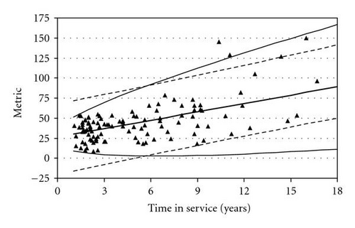
Figure 1 also shows two sets of pointwise 95%-content tolerance intervals constructed at the 90% confidence level. The dashed lines represent the tolerance intervals derived from an ordinary least squares analysis, while the solid lines represent the tolerance intervals derived from an estimated weighted least squares analysis that is described in Section 1.2. The bold line in the figure is the estimated weighted least squares regression line. It is evident in Figure 1 that the ordinary least squares tolerance intervals are inadequate in the sense that they are too wide for small time values and too narrow for large time values. On the other hand, the more pronounced curvature associated with the tolerance intervals derived from the estimated weighted least squares analysis more adequately captures the range of the observations at both ends of the time spectrum.

1.2. Model for Heteroscedasticity

Examination of aerospace data for many part types and many performance metrics led us to propose the following model for heteroscedasticity. Let X(t) denote the metric level at time t for a particular part, and for motivational purposes, assume that the underlying process is a discrete-time valued process (t = 0,1, …). Assume that the initial value of the process is X(0) = β₀ + e, where β₀ is an unknown constant and e is a normally distributed random variable with zero mean and unknown variance . If the degradation process has both a constant deterministic trend, say β₁, and also a random stochastic perturbation, it would follow that X(t) = X(t − 1) + β₁ + s_t, where s_t is a normally distributed random variable with zero mean and unknown variance . It follows from successive substitutions that , or equivalently, X(t) = β₀ + β₁t + e + δ_t, where δ_t is a normally distributed random variable with zero mean and unknown variance . The model for X(t) is (drifting) Brownian motion, except for the fact that the variance function is displaced from the origin by . In our application, the process X(t) is measured one time on each unit; so the data are a collection of independent observations Y_i = X_i(t_i), where X_i(t) is the process associated with the ith unit. Thus, we have the model Y_i = β₀ + β₁t_i + e_i + δ_i (i = 1, …, n) for the observations.

Equivalently, the model implies that observations are independent and normally distributed with means β₀ + β₁t_i and variances . The fact that a variance component, , is responsible for the heteroscedasticity is somewhat unique to our model since the large literature pertaining to heteroscedasticity models usually assumes variances of the form , where h(·) is an arbitrary function (e.g., a polynomial or the exponential function); see [2, 7] and references therein. While these types of models have seen many successful applications, the lucid interpretation of the heteroscedastic variance function was crucial when eliciting buy-in from our aerospace engineering project stakeholders.

1.3. Tolerance Interval for Heteroscedastic Regression

Defining , the log-likelihood function for based on the observations is

()

For a fixed ρ the conditional MLEs, say

and

, of β₀ and β₁ satisfy the linear system of equations:

()

and the conditional MLE of

. The conditional MLEs,

and

, are the weighted least squares estimator of the slope and intercept and have an estimated variance-covariance matrix equal to

, where X is the n × 2 matrix whose first column is all ones and whose second column is the set of values

and Ω(ρ) = Diag(1 + ρt₁, …, 1 + ρt_n).

The profile log-likelihood function (e.g., see reference [8]) of ρ is , which can be maximized to find the MLE of ρ, say . The MLEs of β₀, β₁ and are then are , , and . Unbiasedness of and follows from general results in [9].

A pointwise 100γ%-content tolerance interval with confidence level 100(1 − α)% for a regression line in the context of homoscedastic normal errors was derived in [10]. The following theorem, which is proved in the Appendix A, extends that result to our context.

Theorem 1. If ρ is known, a pointwise 100γ%-content tolerance interval with confidence level 100(1 − α)% for a normal distribution that has mean β₀ + β₁t and variance is

()

where

is the upper 1 − α percentile of a chi-square distribution with n − 2 degrees of freedom and r(ρ) is the solution to

, with N(ρ) = (1 + ρt)/[(1, t)(X^′Ω⁻¹(ρ)X) ⁻¹(1,t)^′].

Proof. See Appendix A.

The pointwise tolerance intervals shown in Figure 1 corresponding to the estimated weighted least squares analysis were drawn from (3) with ρ replaced by its MLE , and with α = 0.1 and γ = 0.95.

1.4. Testing for Heteroscedasticity

Of special importance when analyzing the data for our application is the test of H₀ that the data are homoscedastic. If the hypothesis is not rejected, all the pertinent inference can be drawn from an efficient ordinary least squares analyses. On the other hand, rejecting H₀ protects a practitioner from the pitfalls of using an inappropriate least squares analysis which include a higher than expected false alert rate. Deriving a test for H₀ is particularly interesting from the standpoint that there are alternative tests available in the literature and in subsequent sections in this paper we present a unifying framework for relating alternative tests to each other.

1.5. Overview of Remaining Sections

In Section 2, we position the proposed heteroscedastic model as a special case of a general mixed linear model. We then propose a test of H₀ that is motivated by informally combining the root arguments used when deriving locally most powerful tests and score tests. We show that the test statistic has a distribution that only depends on the underlying variance ratio ρ and thus is amenable to a significance test of H₀ : ρ = 0. A Monte Carlo algorithm for computing the required critical values is outlined. In Section 3, we relate our proposed test to some common tests for heteroscedasticity, namely, the Breusch and Pagan, White, and likelihood ratio tests. In Section 4, we show additional examples of our test for heteroscedasticity and the use of tolerance intervals within the context of aerospace engineering case study. We also report results of a simulation study that examined the power of all the tests that are discussed in this paper. We close the paper with a short summary in Section 5.

2. Proposed Test for Heteroscedasticity

The heteroscedastic regression model developed in Section 1 is a special case of a more general mixed linear model defined by

()

where X is an n × p matrix (we assume without loss of generality that X has a full column rank) of known constants, β is p × 1 vector of fixed-effects, Z is n × m matrix of known constants, s is a m × 1 vector of unobservable random-effects that follow an

distribution, and e is an n × 1 vector of unobservable random error terms, independent of s, and having a

distribution. The special case considered in Section 1 is simply where p = 2 and m = n with Z a diagonal matrix with the values equal to

We begin the derivation of our proposed test for heteroscedasticity by writing the log-likelihood of the general mixed linear model, based on , as follows:

()

Next, there exists an orthogonal matrix Q such that Q^′ZZ^′Q = B, where B is a diagonal matrix whose elements

are the eigenvalues of ZZ^′. It follows that ZZ^′ = QBQ^′, and hence Q^′(I + ρZZ^′)Q = I + ρB. Equivalently, Q^′(I + ρZZ^′) ⁻¹Q = (I + ρB) ⁻¹. Combining this result with the definitions v = Q^′y and μ = Q^′Xβ, the log-likelihood can be rewritten as

()

If β and

were known, the locally most powerful test statistic would be

()

To obtain a useable test statistic we follow the procedure used when deriving the score test (e.g., see [2]) by replacing the unknown β and

by their conditional MLEs given H₀, which are

and

, where r = (I − P_X)y and P_X = X(X^′X) ⁻¹X^′. The resulting statistic is

()

The distribution of r is and by the nature of R it is clear that its distribution only depends on ρ. A simple approach for finding critical values to test H₀ is to simulate r vectors from an MVN_n(0, I − P_X), compute the corresponding values of R from (8), and estimate the critical value from the resulting empirical distribution (edf) function of R values. Denoting the upper-α percentile of the edf by R_a, the R test rejects H₀ if R > R_α. We emphasize the computational simplicity of R, and the ease in which critical values can be obtained. It is also possible to reexpress the null distribution of (8) as a ratio of quadratic forms in independent standard normal random variables and then the saddlepoint approximation described by [11] can be employed to approximate the P-value associated with the test.

A locally most powerful invariant (LMPI) test of H₀ was derived in [12–14]. The derivation of this test is sketched in Appendix B. It can be seen there that the complexity of computing LMPI test is nontrivial. The key result in Appendix B is the demonstration that the LMPI test and the R test are equivalent under the general mixed linear model. The practical significance of this finding is that the computation of the LMPI test, as originally proposed, involves a complicated eigenvalue and eigenvector analysis, whereas computing the equivalent form R test only requires fitting the model with ordinary least squares tools. To characterize this computational contrast another way, the computations associated with the equivalent form R test can be done with software as simple as Excel, whereas the computations associated with the originally proposed form LMPI test will require a rich matrix processing software package.

From a conceptual perspective, the equivalence between the LMPI test and the R test is interesting in the sense that the original complicated derivation of the LMPI test can be replaced by the simpler derivation of the R test. In addition, the demonstrated equivalence also provides further motivation for a procedure introduced in [15] where a test statistic is derived by replacing nuisance parameters in the locally most powerful test statistic by their conditional MLEs. Results in [15] show this procedure produces an asymptotically uniformly most powerful test. Our equivalence finding shows that when we used this approach to derive the R test, in a finite sample context, we arrive at a locally most powerful invariant test.

3. Other Tests for Heteroscedasticity

The Breusch and Pagan test for homogeneity is a partial score test derived for a general setting where the observations are independent and normally distributed with means and variances , where is a p × 1 vector of known covariates, β is a p × 1 vector of unknown parameters, is a q × 1 vector of known covariates (whose components may or may not overlap with the components of ), ξ is a q × 1 vector of unknown parameters, and h(·) is an arbitrary function that is only assumed to possess a first derivative. By setting the first component of to unity, a test of is a test of heteroscedasticity. The Breusch and Pagan test [16] is the partial score test of . For application to our problem, we have , and and the test statistic simplifies to

()

where A is an n × n diagonal matrix whose ith diagonal element is equal to

The White test [17] is positioned to be robust to the normality assumption. For our application, the statistic can be obtained by first computing the vector of squared residuals, say u where , and then computing the test statistic as

()

where J_n is an n × n matrix of ones,

, and V is a matrix whose first column is all ones, whose second column is the values

and whose third column is the values

. Note that the ratio term in the definition of W is simply the R-square value of the regression of u on the V matrix. The distributions of both BP and W depend on ρ and the same Monte Carlo method for approximating the null distribution of R can be used to approximate the null distributions of BP and W.

The log-likelihood function for the general mixed linear model was given in (5) and computation of the MLE of and the conditional MLE of was discussed in Section 2. It follows that the likelihood ratio test statistic is

()

The LRT requires relatively significant computations. For example, computations of the full model MLEs needed by the LRT are not readily available unless software such as PROC MIXED in SAS is available. In standard situations the asymptotic null distribution of LRT is chi-square with degrees of freedom equal to the difference in the dimension of the unconstrained and constrained parameter spaces. However, our situation is not standard since the reduced parameter space lies on the boundary of the unconstrained parameter space. Results in [18] show that the asymptotic distribution of LRT in (11) is a 50: 50 mixture of zero and a chi-square distribution with one degree of freedom. A size-α LRT therefore rejects H₀ : ρ = 0 if

, where

denotes the upper-2α percentile of a chi-square distribution with one degree of freedom.

4. Application to Aerospace Case Study

4.1. Illustrative Examples

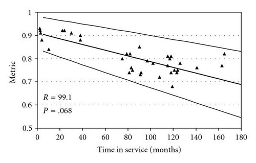
Figure 1 was used in Section 1 as illustrative of a data set that exhibits heteroscedasticity. Figure 2 shows a second illustrative data set (109 observations) which does not exhibit evidence of heteroscedasticity. As in Figure 1, two sets of pointwise 95%-content tolerance intervals constructed at the 90% confidence level are shown corresponding to an ordinary least squares analysis and the estimated weighted least squares analysis described in Section 1.2. In contrast to Figure 1, the two sets of tolerance intervals are nearly identical.

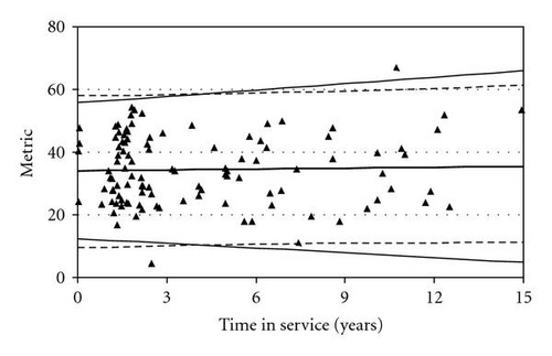
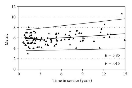
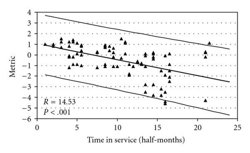
Table 1 shows the computed test statistics R, BP, W, and LRT for the two data sets shown in Figures 1 and 2, along with their P-values for testing H₀ : ρ = 0. The tests all agree that heteroscedasticity appears to exist in Data Set 1 but not in Data Set 2. We note that of all the tests considered, R is by far the simplest to compute with BP and W only slightly more complicated. As described in the introduction, our application context has hundreds of metrics that need to be monitored with this type of analysis methodology. Figures 3, 4, 5, and 6 provide four additional illustrative examples, including the computed R statistic and associated P-value for H₀ : ρ = 0. There is evidence of heteroscedasticity in all four of these data sets.

Table 1. Tests for Heteroscedasticity in Figures 1 and 2.

Test	Data Set
	Data Set 1		Data Set 2
	Statistic	P-value	Statistic	P-value
R	8.92	<.001	4.83	.062
BP	52.1	<.001	2.05	.15
W	26.6	<.001	3.29	.17
LRT	34.8	<.001	1.59	.10

4.2. Power Comparison of Alternative Tests

It is easy to show that the distributions of the R, BP, W, and LRT test statistics depend only on ρ. It follows that the power functions (i.e., the probability of rejecting H₀ : ρ = 0 as function of ρ) of the tests can be evaluated using simulated data sets from the mixed model in (3) using the parameters . We implemented our simulation study using the S-Plus package. For each simulated data set, each of the test statistics can be evaluated and compared to their respective critical values corresponding to nominal size α significance tests. The power of the tests is estimated by the fraction of data sets for which they reject H₀.

Column 2 of Table 2 shows the estimated power of the 10% nominal size R test based on this procedure for ρ ∈ [0,0.25], using 5000 simulated data sets and the same set of values associated with Data Set 1, which is shown in Figure 1. Columns 3–5 of Table 2 give the ratio of the power for the LRT, BP, and W tests, relative to the R test. The results show that the R test and the LRT have nearly identical power, though the R test has slightly better power for small ρ. The R test has uniformly better power than BP and W tests. A somewhat surprising observation is the pronounced dominance of R with respect to BP and W, which are perhaps the two most widely known tests in the economics literature. Table 3 shows similar power comparisons using the associated with Data Set 2, that is shown in Figure 2, and the conclusions are consistent with those drawn from Table 2.

Table 2. Power comparison of the tests using

values from Data Set 1.

ρ	Power of R Test	Ratio of Power Relative to R Test
ρ	Power of R Test	LRT	BP	W
0.00	0.100	0.94	0.91	0.92
0.01	0.155	0.97	0.67	0.67
0.02	0.206	0.97	0.62	0.64
0.03	0.278	1.00	0.63	0.65
0.04	0.344	0.96	0.66	0.60
0.05	0.392	0.99	0.68	0.62
0.06	0.443	1.02	0.68	0.67
0.07	0.492	1.01	0.72	0.67
0.08	0.541	1.01	0.72	0.68
0.09	0.584	1.01	0.77	0.71
0.10	0.624	1.02	0.77	0.70
0.11	0.663	1.02	0.77	0.73
0.12	0.701	1.01	0.80	0.73
0.13	0.719	1.02	0.80	0.73
0.14	0.741	1.03	0.82	0.76
0.15	0.763	1.01	0.84	0.77
0.16	0.783	1.02	0.84	0.78
0.17	0.809	1.01	0.85	0.78
0.18	0.830	1.01	0.86	0.80
0.19	0.830	1.02	0.88	0.82
0.20	0.843	1.02	0.87	0.84
0.21	0.861	1.01	0.88	0.83
0.22	0.869	1.01	0.88	0.84
0.23	0.875	1.02	0.90	0.84
0.24	0.884	1.02	0.90	0.85
0.25	0.900	1.02	0.90	0.85
0.30	0.923	1.01	0.93	0.89
0.35	0.943	1.00	0.94	0.92
0.40	0.949	1.01	0.96	0.93

Table 3. Power comparison of the tests using

values from Data Set 2.

ρ	Power of R Test	Ratio of Power Relative to R Test
ρ	Power of R Test	LRT	BP	W
0	0.100	1.01	0.96	0.89
0.001	0.107	0.95	0.91	0.84
0.002	0.104	1.01	0.90	0.98
0.003	0.126	0.92	0.78	0.75
0.004	0.127	0.96	0.72	0.81
0.005	0.128	0.92	0.75	0.68
0.006	0.134	1.00	0.70	0.81
0.007	0.146	0.84	0.65	0.65
0.008	0.136	1.03	0.78	0.76
0.009	0.137	1.06	0.78	0.77
0.010	0.148	0.90	0.73	0.68
0.011	0.152	1.01	0.72	0.78
0.012	0.174	0.86	0.65	0.68
0.013	0.171	0.97	0.68	0.73
0.014	0.168	1.03	0.68	0.74
0.015	0.183	0.92	0.63	0.70
0.016	0.189	0.93	0.69	0.67
0.017	0.200	0.92	0.63	0.65
0.018	0.204	0.92	0.65	0.62
0.019	0.205	0.99	0.67	0.65
0.02	0.206	0.99	0.64	0.64
0.03	0.267	0.98	0.66	0.61
0.04	0.316	1.10	0.66	0.64
0.05	0.384	0.85	0.71	0.63
0.06	0.443	1.01	0.71	0.63
0.07	0.496	1.02	0.74	0.64
0.08	0.544	1.02	0.74	0.68
0.09	0.586	1.03	0.76	0.70
0.10	0.639	1.00	0.76	0.68
0.11	0.676	1.01	0.80	0.71
0.12	0.700	1.01	0.82	0.72
0.13	0.735	1.01	0.83	0.77
0.14	0.756	1.02	0.84	0.77
0.15	0.783	1.01	0.84	0.79
0.16	0.799	1.01	0.87	0.81
0.17	0.828	1.00	0.85	0.80
0.18	0.830	1.03	0.87	0.82
0.19	0.853	1.01	0.89	0.83
0.20	0.868	1.01	0.89	0.84
0.21	0.878	1.01	0.90	0.85
0.22	0.887	1.01	0.91	0.86
0.23	0.897	1.01	0.91	0.86
0.24	0.903	1.02	0.92	0.89
0.25	0.907	1.03	0.93	0.89
0.30	0.935	1.02	0.95	0.92
0.35	0.959	1.01	0.96	0.94
0.40	0.973	1.01	0.96	0.95

5. Summary

Our aerospace case study, which pertains to the time evolution of performance metrics for electronic equipment, motivated the derivation of a model for heteroscedastic regression errors. A test for homoscedasticity was proposed and compared with various other tests that are prevalent in the literature. The proposed R test was shown to be equivalent to an LMPI test associated with a general mixed linear model of which this paper’s heteroscedastic regression model can be regarded as a special case. Aside from what we judge to be a simpler intuitive motivation associated with the R test formulation, it has the practical benefit of being much simpler to compute than the formula that results from the classical LMPI derivation. The power of the R test was compared to some popular alternative tests, and only the considerably more difficult to compute likelihood ratio test has power that is comparable to the R test. We extended the classical application of tolerance intervals for regression to our heteroscedastic case and illustrated their use with six data sets from our aerospace case study.

Appendices

A. Tolerance Intervals for Heteroscedastic Model

Using observations that follow a simple linear regression model Y_i = β₀ + β₁t_i + e_i, (i = 1, …, n), Wallis [10] derived a tolerance interval for a normal distribution that has mean β₀ + β₁t and variance . The Wallis interval easily extends to the more general case where the observations are of the form Y_i = β₀t_0i + β₁t_1i + e_i, where the are not necessarily equal to unity. In particular, a 100(1 − α)% tolerance interval with content γ for the normal distribution with mean β₀t₀ + β₁t₁ (where t₀ and t₁ are arbitrary) and variance is

()

where

and s² denote the ordinary least squares estimates of (β₀, β₁) and

using an X matrix that has the values

in its first column, rather than unity, and moreover, when computing the r value from

()

where

The heteroscedastic regression model described in Section 1.2 generalizes the problem solved by Wallis by having independent and normally distributed with zero means and variances equal to , where ρ is a new parameter. The derivation in this Appendix is for the case where ρ is known so that the observations can equivalently be expressed as

()

where

are independent and normally distributed with zero means and variances equal to

. Defining

and

, it follows that a 100(1 − α)% tolerance interval with content γ for a normal distribution with mean β₀t₀ + β₁t₁ and variance

()

where

with

being the n × 2 matrix whose first column is the values

and whose second column is the values

, and where r(ρ) is the solution r to (A.2) but with N replaced by

Referring back to Section 1.2, it is easily seen that = and = . For the particular choice (t₀, t₁) = , it can also be shown that N(ρ) = (1 + ρt)/[(1, t)[X^′Ω⁻¹(ρ)X] ⁻¹(1,t)^′] and (A.4) becomes

()

Finally, by multiplying the endpoints of (A.5) by

a 100(1 − α)% tolerance interval with content γ for a normal distribution that has mean β₀ + β₁t and variance

is obtained. The resulting interval has the form

()

as reported in Section 1.3.

B. Equivalence of R Test and LMPI Test

Following [19], where P_XZ = [X : Z]([X:Z]^′[X : Z]) ⁻¹[X:Z]^′, an appropriate ANOVA table for the mixed model is based on the sum-of-squares decomposition y^′y = y^′P_Xy + y^′(P_XZ − P_X)y + y^′(I − P_XZ)y. The first two terms on the right-hand-side of this decomposition, which we denote as S_β and S_s, respectively, correspond to fitting the fixed-effects first and then fitting the random-effects after the fixed-effects. The final term, denoted as S_e, corresponds to the residual error sum-of-squares. It can be shown that the degrees of freedom associated with these three quadratic forms are p, r = rank (X : Z) − rank (X) and f = n − rank (X : Z), respectively.

Let the nonzero eigenvalues of C = Z^′(I − P_X)Z be denoted by Δ₁ ≤ Δ₂ ≤ ⋯≤Δ_r, and define D = diag (Δ_i). Let d denote the number of distinct eigenvalues of C, and denote their values by and their multiplicities by . Define Q to be the m × r matrix of orthornormal eigenvectors corresponding to the . Finally, let q = Z^′(I − P_X)y and define to be a solution to . The following results are proved in [19].

(a)
has a
(b)
is independent of S_e.
(c)
For (note that the cardinality of J_i is r_i) and , S_s(i) are independent with and .

It is shown in [12] that the locally most powerful invariant test statistic for testing H₀ is

()

Although S_e explicitly appears in the denominator of (B.1), use of the LMPI test does not require f > 0. For the cases where f = 0 (S_e = 0), such as what will occur with our application since Z is a diagonal matrix of rank n, the LMPI test is still useable with the test statistic simply reducing to

. Alternative derivations of the LMPI test were proposed in [14, 15].

To prove the equivalence of the LMPI test based on (B.1) and the R test based on (8), we first note that S_e + S_s = y^′(I − P_XZ)y + y^′(P_XZ − P_X)y = y^′(I − P_X)y = r^′r, which establishes the denominator of the two test statistics coincide. Next, we observe that the numerator of LMPI test statistic, , can be reexpressed as . Since C = QDQ^′ implies C² = QD²Q^′, we have t^′Dt = = q^′q = y^′(I − P_X)ZZ^′(I − P_X)y = r^′ZZ^′r, which establishes that the numerators of the two statistics are also identical.

References

1 Piepel G. F., Cooley S. K., and Paul M. R., Upper tolerance intervals adjusted for multiple nuisance uncertainties, Journal of Quality Technology. (2008) 40, no. 3, 245–258, 2-s2.0-47149113989.
Google Scholar
2 Davidson R. and MacKinnon J. G., Estimation and Inference in Econometrics, 1993, Oxford University Press, New York, NY, USA.
Google Scholar
3 Cohen J., Cohen P., West S. G., and Aiken L. S., Applied Multiple Regression/Correlation Analysis for the Behavioral Sciences, 2003, 2nd edition, Lawrence Erlbaum Associates, Hillsdale, NJ, USA.
Google Scholar
4 Gelman A. and Hill J., Data Analysis Using Regression and Multi-Level/Hierarchical Models, 2007, Cambridge University Press, New York, NY, USA.
Google Scholar
5 Barnett V., Environmental Statistics: Methods and Applications, 2004, John Wiley & Sons, New York, NY, USA.
Google Scholar
6 Leedan Y. and Meer P., Heteroscedastic regression in computer vision: problems with bilinear constraint, International Journal of Computer Vision. (2000) 37, no. 2, 127–150, https://doi.org/10.1023/A:1008185619375, 2-s2.0-0034206736.
Google Scholar
7 Carroll R. J. and Ruppert D., Transformation and Weighting in Regression, 1988, Chapman & Hall, New York, NY, USA.
Google Scholar
8 Berger J. O., Liseo B., and Wolpert R. L., Integrated likelihood methods for eliminating nuisance parameters, Statistical Science. (1999) 14, no. 1, 1–28, 2-s2.0-0002464001.
10.1214/ss/1009211804
Google Scholar
9 Kackar R. and Harville D. A., Approximations for standard errors of estimators of fixed and random effects in mixed linear models, Journal of the American Statistical Association. (1984) 79, 853–862.
Google Scholar
10 Wallis W. A., Tolerance intervals for linear regression, Proceedings of the 2nd Berkeley Symposium on Mathematical Statistics, 1951, 43–51.
Google Scholar
11 Lieberman O., Saddlepoint approximation for the distribution of a ratio of quadratic forms in normal variables, Journal of the American Statistical Association. (1994) 89, 924–928.
Google Scholar
12 Lin T. and Harville D. A., Some alternatives to Wald′s confidence interval and test, Journal of the American Statistical Association. (1991) 86, 179–187.
Google Scholar
13 Nyblom J. and Makelainen T., Comparisons of tests for the presence of random Walk coefficients in a simple linear model, Journal of the American Statistical Association. (1983) 78, 856–864.
Google Scholar
14 Westfall P. H., Power comparison for invariant variance ratio tests in mixed ANOVA models, The Annals of Statistics. (1989) 17, 318–326.
Google Scholar
15 Marohn F., A comment on locally most powerful tests in the presence of nuisance parameters, Communications in Statistics: Theory and Methods. (2002) 31, no. 3, 337–349, 2-s2.0-34548177301.
Google Scholar
16 Breusch T. S. and Pagan A. R., A simple test for heteroscedasticity and random coefficient variation, Econometrica. (1979) 47, 1287–1294.
Google Scholar
17 White H., A heteroskedasticity-consistent covariance matrix estimator and a direct test for heteroskedasticity, Econometrica. (1980) 48, 817–838.
Google Scholar
18 Self S. G. and Liang K., Asymptotic properties of maximum likelihood estimators and likelhood ratio tests under nonstandard conditions, Journal of the American Statistical Association. (1987) 82, 605–610.
Google Scholar
19 Harville D. A. and Fenech A. O., Confidence intervals for a variance ratio, or for heritability, in an unbalanced mixed linear model, Biometrics. (1985) 41, no. 1, 137–152, 2-s2.0-0022267760.
Google Scholar

All articles

Tolerance Intervals in a Heteroscedastic Linear Regression Context with Applications to Aerospace Equipment Surveillance

Abstract