Examination of Particle Tails

1. Introduction

This paper focuses on the effective sampling distribution of particle swarm optimisation (PSO). PSO is a population-based global optimisation technique. The algorithm is made of two essential steps: particle movement (dynamics) through a search space of solutions and an indirect particle interaction which is mediated by information sharing within a social network. Particles place personal “attractors" in the search space at positions corresponding to the best location (as determined by the evaluation of an objective function) that they have visited. The dynamical update rule which specifies the acceleration of a particle i is a sum of an attraction towards a personal attractor and an attraction towards the best attractor amongst other particles in i′s social neighbourhood [1–3]. The particle acceleration is added to particle velocity in a discretisation of particle kinematics; the velocity is added in turn to particle position and a new trial solution is achieved. Despite the simplicity of this scheme, the algorithm is effective over the standard benchmark problems and has increasing numbers of real-world applications. However, little is known about how a PSO achieves its results.

The sampling distribution provides the probability density of particle placement between and around fixed attractors. This scenario occurs when the swarm “stagnates," the swarm is not improving, the network of attractors is fixed, and the particles are moving independently of each other, that is, the particles decouple. Stagnation can occur in the full model, or can be imposed for the purposes of the oretical analysis. In general, particles are expected to search in the immediate vicinity of the attractors, and indeed this behaviour is necessary for convergence. The central portion of the sampling distribution is therefore coincident with this region. However, the swarm must retain an ability to explore outside the attractor vicinity if premature convergence, a problem in complex environments, is to be avoided. This exploration is due to the finite tail of the sampling distribution; there is a small probability that a particle will be displaced far from the region of convergence, and this probability increases with tail fatness.

Some insights into the PSO sampling distribution have been provided by a study of “bare bones" formulations [4]. In this work, Kennedy replaced the particle update rule with sampling from a Gaussian distribution with mean at the centroid of the personal and neighbourhood best positions of each particle, and standard deviation was set to the separation between them. Performance comparisons with a few benchmark problems were disappointing (later confirmed in [5]), but the addition by hand of particle “bursts" ameliorated the situation somewhat, indicating that the tails of this Gaussian distribution function are too thin to enable escape from stagnation. Further evidence for this conclusion has been provided by a study of Lévy bare bones [5] where more extensive trials showed that fat tails, as provided by the Lévy distribution, improve bare bones performance so that it becomes effectively equivalent to standard PSO. A recent theoretical analysis of bare bones PSO has been given in [6]. However, a Gaussian bare bones version of a “fully informed" particle swarm (FIPS) was able to deliver good performance over a small testbed of functions [7], which suggests that particle tails might not be so important, at least for FIPS.

It is known that decoupled PSO exhibits bursts of outliers [8]. Bursts are temporary excursions, along a coordinate axis, of the particle to large distances from the attractors. A burst will typically grow to a maximum and then return through a number of damped oscillations to the region of the attractors. The addition of bursts to Gaussian bare bones increases the chance of particle displacement away from the attractors, fattening the tail of the overall sampling distribution. Lévy distributions also produce particle outliers, but these outliers are not correlated; they do not occur in sequence along a single axis. At the moment, the circumstances, when a sequence of correlated outliers (as manifest, for example, in PSO bursts) might prove to be fortuitous, are unknown. This paper investigates the tail of the PSO sampling distribution. Our results show that this tail is described by power laws and is therefore fatter than Gaussian. This fattening is indeed due to bursting, the origin of which is concluded to lie in a process known as multiplicative randomness.

Bursting is already known to occur in first-order stochastic difference equations [9]. This paper generalises the first order results to second order difference equations with multiplicative randomness, a class of equations that includes standard PSO. Since the amount of bursting is dependent on the range of the probability distributions, the paper begins by discussing possible parameter regimes. This is accomplished by a formulation of PSO as a finite difference equation. The paper continues with a series of experiments which reveal the power law tails of the sampling distribution. Section 4 introduces multiplicative randomness and power law tails in first-order processes and extends these results to second-order difference equations. A competitive reformulation PSO without multiplicative randomness has recently been proposed (recombinant PSO, [10]). Section 5 investigates decoupled recombinant PSO and demonstrates the consequent thinness of the distribution tail. The results of this paper are drawn together in a concluding section and some open research questions are outlined.

2. PSO and Stochastic Difference Equations

This section recasts PSO as a stochastic difference equation (SDE). Since this is an unfamiliar form of PSO, a few relations from the literature governing parameter choice are gathered together and presented here.

Poli and Broomhead [19] has extended this analysis by retaining randomness and deriving stability relations for the expectations of the first and second moments of position. The relation for the expected value of x is equivalent to the above analysis with u = 0.5, so the upper bound on the acceleration parameters ϕ is therefore twice the u = 1 bound.

As ϕ^CK → 4, χ → 1, the system becomes unstable, and as ϕ^CK grows from 4, χ decreases from 1 and the system is increasingly damped. In terms of the inertia weight formulation, these parameters correspond to w ≈ 0.73 and ϕ_IW ≈ 3.0. Many trials of PSO over commonly used test functions have found that best performance is attained at ϕ close to the u = 1 stability condition. The reason behind this can be elucidated by considering the statistical distribution of x(t).

3. Distribution Tail

This section presents an experimental investigation of the tail of sampling distribution for decoupled PSO. In each experiment described here, x(1) and x(2) are random starting positions between the two fixed attractors, p₁ = −0.5 and p₂ = 0.5. Henceforth, only the IW form of PSO will be considered (the Clerc-Kennedy form is a simple parameter redefinition) and the suffix IW will be dropped for ease of notation.

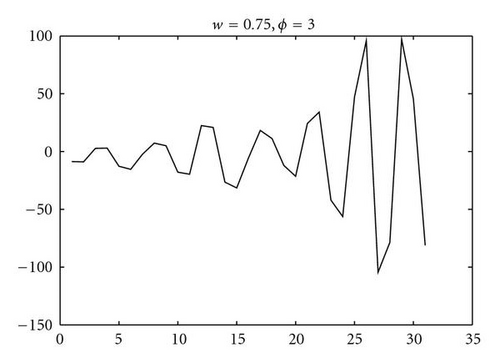
Figure 1 shows the development of a spectacular burst for the system defined by (9) at w = 0.75, ϕ = 3.0. The particle is close to the u = 1 instability condition since, from (11), ϕ_max = 3.5. Figure 1 shows a burst of two orders of magnitude, as measured in units of the intrinsic scale |p₁ − p₂|.

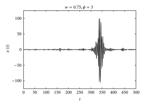
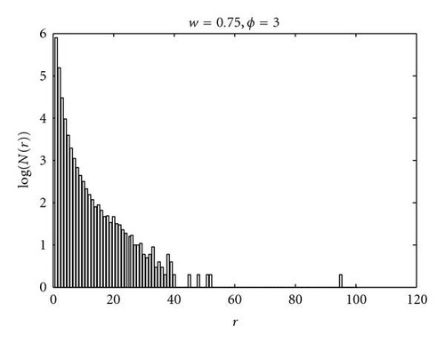
Figure 2 shows the frequency N of particle distance r = |x| for the same system as Figure 1 for a run of 10⁶ iterations. A logarithmic scale (all logs in this paper are to base 10) has been used for the y-axis so that the infrequent but large bursts are visible on the plot. For this single run, the mean distance was 0.747 (standard deviation 1.05) and all distances are in the interval [1.01 × 10⁻⁶, 105]. Many updates are therefore over very small distances from the origin, which is the fixed point 〈c〉/(1 + 〈a〉+b) of the expectation value of x. Although the standard deviation is of the order of the attractor separation, r can range over 8 orders of magnitude.

Bursts would be expected to fatten the tail of the particle distance distribution p(r) when compared to distributions with exponential falloffs such as a Gaussian. Evidence for possible power law fattening of the distribution tail, p(r)  ~  r^−α, where p(r)dr is the probability of a particle at distance r, would be revealed in a plot of the logarithm of the cumulative distribution function, P(r), where P(R) = prob (r > R). A cumulative plot (also known as a rank/frequency plot [20]) reduces sampling errors in the tail of the plot, even with logarithmic binning [21]. A relation p(r)  ~  r^−α corresponds to P(R)  ~  r^1−α and a plot of log (P) against log (r) would show a straight line with gradient 1 − α.

Figure 3 shows cumulative distributions for 50 runs of 10⁵ iterations, once more for the decoupled PSO defined by w = 0.75, ϕ = 3.0, p_1,2 = ± 0.5,  x(1),  x(2) = U(p₁,p₂). All runs have been plotted on this figure to give an idea of the deviations between runs. The straight portion in Figure 3 is evidence for a power law (although the underlying distribution might be log-normal; see discussion in the following paragraphs).

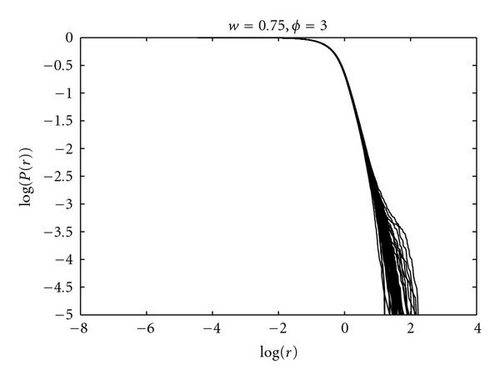
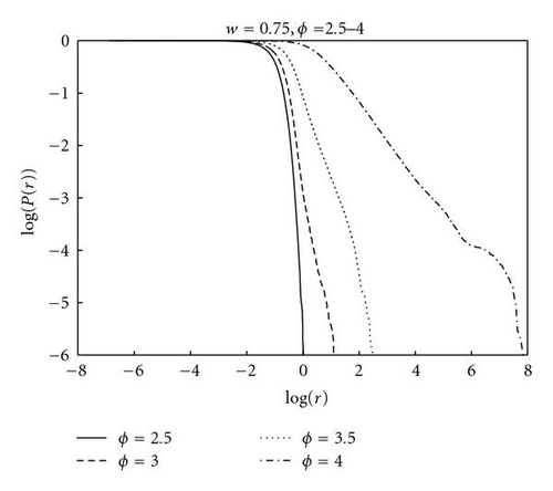
Figure 4 shows cumulative probability distribution plots for four values of ϕ at w = 0.75. This data is collected over 50 runs of 10⁶ iterations for each value of ϕ. Each line shows a straight central part. The lines curve inwards towards the end of the sample where probabilities are small (<10⁻⁵) and there are just a few events. Once more, a large part of the distribution is concentrated in the region between the attractors, r < 1. The power laws become established by r ≈ 1.0, the separation of the attractors. At ϕ = 4.0 the power law is evident for some 4 orders of magnitude.

Putative power laws as revealed by log-log plots are hardly distinguished from log-normal laws p(x)  ~  exp (−ln (x − μ) ²) over four or less orders of magnitude [21]. These plots therefore only show that the tails might be modelled by a power-law distribution. The underlying distribution could be power law or another distribution, such as the log normal, whose tail can be approximated by a power law over some range.

Figure 5 plots the same data as Figure 4 but over the interval 10⁻⁴ < P(r) < 10⁻¹ where the power laws are becoming established. For clarity, every 1000th r in this range has been plotted. The gradients and correlation coefficients of the four lines are −3.94(−0.987), −3.74(−0.998), −1.08(−0.999), and −0.73(−0.999) for ϕ = 2.5, 3.0, 3.5, 4.0, respectively. (A correlation coefficient of −1.0 indicates perfect negative correlation.)

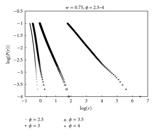
If the sampling distribution p(r) does follow a power law falloff, p(r)  ~  r^−α for r > r_min (as these results suggest), then 〈r〉 is well defined only for α > 2 because $$ diverges for α < 2. According to these experiments, at ϕ = 3.5, the tail falls off as p  ~  r^−2.08, so 〈r〉 is finite at this value (and at smaller values) of ϕ, but 〈r〉 diverges at larger values. This edge is just at the u = 1 stability condition. Lower values of u, and hence higher values of ϕ, lead to systems whose empirical mean over a finite number of iterations will be finite but will nevertheless vary enormously, sometimes taking on large values, in order to respect the formal divergence of the mathematical mean.

From the condition P(r) = 0.1, Figure 5 shows that 10 per cent of the particle positions are at distances greater than 0.21, 0.32, 0.92, and 56.8 from the origin for ϕ = 2.5, 3.0, 3.5, and 4.0, respectively. This indicates that good coverage of the region p₁ < r < p₂ is attained for ϕ = 2.5, 3.0 and 3.5. On the other hand, there is no coverage outside this interval for ϕ = 2.5, showing that this PSO concentrates all its search between the attractors. At ϕ = 3.0, particles will move outside this region, enhancing exploration away from the fixed points in the interactive model (where p₁ and p₂ can be updated). At ϕ = 3.5, 4.0, the frequent bursts often take r far from the attractors. These large bursts cannot help with convergence, but they might help diversify the fully coupled system.

An analysis of the data for the 50 runs at ϕ = 4.0,w = 0.75 found a probability of 10 per cent for positions of at least 10⁴⁰. ϕ = 4.0 is between the u = 1 and u = 0.5 stability conditions (3.5 and 7.0, resp.). Although none of these runs exploded, bursts of extremely high amplitude were common. The inference from these experiments is that the u = 1 stability condition corresponds to power law tails with bounded mean. Moving ϕ beyond the u = 1 condition leads to unbounded mean displacements and little exploration of the region between the attractors. This may explain the popular empirical choices w ≈ 0.73 and ϕ_IW ≈ 3.0.

4. Multiplicative Randomness

(This is in contrast to a bare bones formulations which sample from a probability distribution N. N might itself has fat tails but outliers need not be correlated and arbitrarily large steps r(t + 1) − r(t) are possible. Bursts are a feature of the finite difference equations.)

The previous section presented an evidence that the decoupled PSO shows power-law behaviour when close to constant-u instability. Power-law tails are found in many natural systems. Well-known examples include the distribution of earthquake magnitudes, frequency of words in a language, wealth of the richest people, and physical quantities close to a phase transition. Although power laws have been regarded as an indicator of self-organisation (e.g., [22]), this explanation is not necessary [21, 23].

Other possible explanations of bursts include resonance. Certainly, (3) has a driving term c(t) and a spring-like term Φ(t)(p_i − x(t)), (1), and might be expected to resonate. However, the system does not have a well-defined resonant frequency because the spring constants Φ are themselves random.

Intermittent chaotic systems show periods of constant amplitude punctuated by erratic bursts [24]. However, decoupled PSO is not chaotic in the stable regime. Another simpler explanation for power laws can be found in the theory of random multiplicative processes [9].

4.1. First-Order SDE

Considering the first order SDE

$$ (18)

then x(t) = (−) ^ta(t − 1)a(t − 2) ⋯ a(0)x(0). The distribution of x is therefore given by the distribution of products of random numbers. The logarithm of x(t) is equal to a sum of logarithms of random numbers, and by the central limit theorem, the distribution of log (x) will be normal. The distribution of x(t) is therefore log normal, and log-normal laws are well approximated by power laws over intervals of four or less orders of magnitude [21]. This simple argument shows that fat, power-law tails can derive from first-order multiplicative processes.

However, (18) is a very poor approximation to PSO. The second-order SDE defined by (3) reduces to the first-order SDE considered above for b = 0, c(t) = 0. This corresponds to a PSO with w = 0 and ∑Φ_ip_i = 0. This implies that u₁ = u₂ and p₁ + p₂ = 0; giving a PSO,

$$ (19)

where u₃ is a random value. (19) was tested over a suite of 14 objective functions, duplicating the test conditions of [11], with very poor results.

The first-order SDE with additive noise,

$$ (20)

has been studied by Sornette and other workers (e.g., see [9] for a(t) < 0). This system contains both multiplicative a(t) and additive c(t) randomness. Decoupled PSO reduces to (20) if the inertia weight is set to zero, w = 0,

$$ (21)

Once more, performance of the fully coupled version of (21) is very poor over the above test function set. Without velocity, these PSOs cannot move through the search space and are doomed to local exploration around the initial particle configuration.

Equation (20) exhibits a regime of power-law behaviour. With c(t) = 0, we recover model (18) which is log normal in its central part [25]. For c finite, iterating (19) gives the solution of (19) as

$$ (22)

which shows that the fate of x is determined by the multiplications over a. The surprising feature is that (21) exhibits interesting behaviour in the stable regime 〈a〉<1 [9]. This behaviour, namely intermittent bursts and power law tails to the distribution of x, is contingent on max (a(t)) > 1 so that amplification is possible, and upon the injection of noise, c ≠ 0 so that convergence to the fixed point is prevented.

Rewriting the w = 0 PSO as

$$ (23)

facilitates the comparison with (20). The fixed- u stability condition is 0 < ϕu < 2. Without loss of generality, we can place p₁ = 1.0, p₂ = 0 so that c(t) = (ϕ/2)u₁. From the u = 1 stability condition, ϕ < 2, c(t)  ~  U(0, c_max), c_max < 1. Furthermore, a(t)∈[−1,ϕ], although the distribution within this interval is triangular rather than uniform. This means that the w = 0 PSO differs from (20) in two respects: a(t) can become positive and c and a are not independent. Indeed, a(t) = [c(t) + (ϕ/2)u₂ − 1].

These changes were investigated by trials on Sornette and Cont′s original system, (20) with a  ~  U(a_min,a_max) and c(t)  ~  U(0, 1). The results are shown in Figure 6. The plots depict average distances r = |x| from the origin over 50 runs of 10⁶ iterations and show results for four uniform distributions of a, each with |〈a〉| < 1.0 and max (|a | > 1). Line (i), a  ~  U(−1.48, − 0.48), corresponds to the system previously studied by Sornette and Cont [26], line (ii), a  ~  U(−1.5,1.5), is a symmetrical distribution with 〈a〉 = 0, and line (iii), a ~ U(−1.75,1.25), has 〈a〉 = −0.25.

The plot shows the fat power-law tail for the Sornette-Cont system. The results also show thin tails when the mean a is close to zero (lines (ii) and (iii)). This can be explained by the relative drop in probability of amplification, |a | > 1. In SDEs (ii) and (iii), prob (|a | > 1) = 1/3, whereas in the Sornette-Cont system, prob (|a | > 1) = 0.48. The second term of (22) can be ignored during a large burst |x(n)|≫|x(0)| ≫ max (c),

$$ (24)

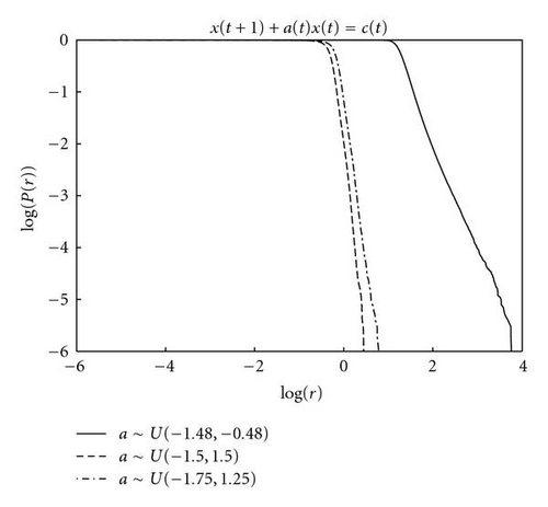
Sequences of a(l) with large products will occur less often in (ii) and (iii) compared to (i), and the distribution tail is quenched. A comparison of SDEs (ii) and (iii) reveals a slightly fatter tail for (iii). This is because max (|a|) is larger in this system, and amplification is increased because products of a′s of a given length n, $$, can attain higher values.

In summary, power-law tail behaviour is possible in first-order SDEs, although the fatness of the tail will depend on the choice of parameters; fattening bursts are possible if max (|a|) > 1 and the distribution assumes a power-law tail for finite c. Standard PSO is badly approximated by a first-order SDE (however, a novel first-order PSO variant, a simplified version of recombinant PSO, does produce good search behaviour [27]). The next section examines second-order SDEs which provide a much closer model of standard PSO.

4.2. Second-Order SDE

The second-order stochastic system with uniform distributions

$$ (25)

has not, to our knowledge, been studied in the burst regime max (|a|) > 1. (25) is closely related to the decoupled PSO with p₁ = 1, p₂ = 0:

$$ (26)

Replacing u₁ + u₂ with a uniform distributions leads to

$$ (27)

and in particular, for the ϕ = 3.0, w = 0.75 system,

$$ (28)

Figure 7 shows the cumulative distribution r = |x| for (28) for 50 runs of 10⁶ iterations. Comparison with the first-order SDEs of Figure 6 shows that this second-order SDE has very fat tails with 10% of all positions at distances of 4 × 10⁵ or more from the origin. The frequent and large bursts are not well modelled by a power law.

This behaviour is in contrast to the decoupled PSO of (26), plotted in Figure 3, which shows a very much more restrained tail. The principle difference between (26) and (28) is the replacement of the triangular-shaped random number distribution by a uniform distribution. Although 〈a〉 and max  (|a|) are identical, the uniform distribution increases prob (|a | > 1), leading to an increased probability of large products $$.

The contribution of such products to a burst can be seen by formally deriving a solution for x(t) as a sum over products of random variables. Rewriting (25) as

$$ (29)

where L is the lag operator Lx_j = x_j−1, L²x_j = x_j−2, La_j = a_j−1L, a(t) = −a_j, and iterating back in time,

$$ (30)

Hence, after m iterations,

$$ (31)

Equation (31) reduces to the solution of the first-order difference equation, (22), for m = n, b = 0.

During a large burst |x_n | ≫ x_n−2m ≫ max (c),

$$ (32)

which shows that the amplification of the burst is enhanced compared to a first-order burst (24), by the terms in b. The validity of this remark depends on the relative sign of each term appearing in (32). To estimate just how big the enhancement might be, suppose that all the a′s are positive and the x′s alternate in sign. The probability distribution function P_m(A) of the product of the random multipliers A = a₁a − 2 ⋯ a_m is approximated by $$ (see, e.g., [9]) for large A, where p(a) is the distribution of a. Then, for large A, we can replace each random variable a in (31) by the geometric mean $$. This gives an upper bound to x_m, $$ where (by assumption) x_n−1 > x_n−2m. This second order burst is boosted in comparison to a first-order burst $$. Although such large bursts will be rare, they will contribute to the overall probability distribution of x because, although exponentially unlikely, they are of exponential size (see, e.g., the argument of Redner [25] for the product of a binary sequence xyxxyxyy).

The oscillatory pattern of any large burst can be deduced by considering x_n+1 = a_nx_n − 0.75x_n−1 where |x_n+1 | >|x_n | >|x_n−1 | ≫ max (c). Suppose, for the sake of argument, that x_n−1 is positive. Then |x_n+1| will be maximised if a_nx_n < 0 with the result x_n+1 < 0. Hence, x_n+1 and x_n−1 differ in sign. x_n might be positive or negative; in either case, we expect x_n+2 to be of the reverse sign in a large burst. The conclusion is that large bursts are likely to follow a pattern sign (x) = {++−−++−−} as demonstrated in a close-up of the burst of Figure 8.

5. Additive Randomness

Figure 9 reports on the cumulative distribution of particle separation r for (33). The distributions for w = 0.5 and various ϕ up to the maximum stable value of ϕ = 3.0 were collected for 50 runs of 10⁶ iterations with x(1),x(2) ~ U(−0.5,0.5), p₁ = −0.5,  p_l = 0.5,  p_r = 1.0.

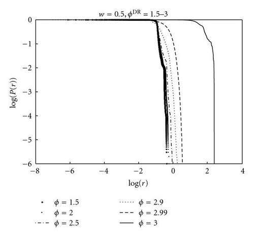
The cumulative distributions are flat for small r, and then drop vertically at a cutoff r − c, suggesting p(0 ≥ r ≥ r_c) = U(0, r_c) (although the log-log plot is not sensitive enough to show variations from uniformity). The noncritical systems ϕ ≤ 2.9 place the majority of the positions between the attractors. At subcriticality, ϕ = 2.99, the system is inclined to explore beyond the attractors, r_c > 1. At instability, r_c is between 50 and 100. A vertical drop-off beyond r_c would be an evidence that additive-SDE does not develop tails, and this is confirmed by these plots, except perhaps for ϕ = 2.99 which appears to have a finite, but very large slope.

In fact, PSO models such as (33) might produce tails from a resonance effect. This is because the spring constants are fixed and the system has a defined natural frequency. For the case of PSO-DR, setting p₃ = (p₁ + p₂)/2 gives a simple oscillator with force law F = ϕ(p₃ − x) and natural frequency $$. The periodic time, T = 2π/ω for ϕ = 1 (this is empirically a good value for interacting PSO-DR [28]), is therefore about 6 with the implication that an oscillating p₃ on the timescale of 6 iterations could drive the oscillator and amplify x. This could happen from a shifting neighbour best position p₁, or from an oscillation between p_l and p_r in the p₂ term, or by a combination of the two.

6. Conclusions

This paper has investigated the position distribution of decoupled PSO. Particular attention has been paid to the tail of this distribution, a regime dominated by power laws. The origin of these tails lies with the phenomenon of particle bursts. Bursts occur at all scales with decreasing probability for increasing size. The accumulation of bursts of all sizes results in distribution tail fattening. In order to study how these bursts might develop, decoupled PSO has been formulated as a second-order stochastic difference equation. Fat distribution tails, well modelled by power laws (although the underlying distribution might be log normal, or some other distribution with a power-law regime), arise from multiplicative randomness, a phenomenon previously encountered in first-order SDEs, and generalised here to second order processes.

This conclusion is valid for first- or second-order SDEs where the multiplicative random variable a is capable of amplification (max (|a|) > 1), but does not permit system explosion (〈|a | 〉<1). According to the theoretical analysis presented here, bursting in a second-order SDE is built from a sum of multiplicative stochastic processes, and the burst size is boosted by the second-order parameter b. This result explains the observation that the particle distribution shifts as more iterations are collected. The distribution is dominated by large but rare events that are only manifest after many iterations.

A stability condition for the PSO parameters w and ϕ can be achieved by replacing the random variables in the difference equation by a constant u. The inference from a set of experiments is that the u = 1 stability condition leads to power-law tails with bounded mean. Moving ϕ beyond this condition leads to unbounded mean displacements. The popular ϕ = 3.0,w = 0.75 PSO, is within the stable region and has weak power-law tails, which enhance exploration, yet also has good coverage of the region close to the attractors, enabling convergence.

There is a tantalising possibility that the removal of stochasticity from the dynamics might render PSO amenable to further theoretical analysis. A recombinant PSO, which is demonstrably competitive to standard PSO, almost achieves this miracle. The acceleration parameters are constant in PSO-DR, but randomness, and hence diversity regeneration, is manifest in a jiggling of the attractor components. This jiggling will persist even at times of stagnation. PSO-DR, replete with just additive randomness of this sort, does not, according to the theoretical and empirical arguments supplied here, enjoy bursting activity. It is conjectured that this transfer of randomness from the dynamics to the information network generates enough noise to mitigate against premature convergence in the coupled model, despite the thin tails of the decoupled equations. These issues are taken up in [27, 28]. (See also [29].)

PSO bursts differ from the outliers generated by bare bones swarms in two respects: the outliers occur in sequence, and they are one dimensional. Bursting will therefore produce periods of rectilinear motion where the particle will have a large velocity parallel to a coordinate axis. Whether bursts are generally beneficial, or a hindrance, to a fully interactive PSO and under what circumstances, is the subject of ongoing research [28]. What does appear to be certain is that a distribution of outliers which decreases slower than a Gaussian tail is important if PSO is to escape premature convergence in difficult environments. Standard PSO achieves this through multiplicative randomness and this occurs even in the decoupled system; recombinant PSO can only, however, gain its outliers through the interaction of the particles.