We have previously proposed a hybrid particle swarm optimisation/ant colony optimisation (PSO/ACO) algorithm for the discovery of classification rules. Unlike a conventional PSO algorithm, this hybrid algorithm can directly cope with nominal attributes, without converting nominal values into binary numbers in a preprocessing phase. PSO/ACO2 also directly deals with both continuous and nominal attribute values, a feature that current PSO and ACO rule induction algorithms lack. We evaluate the new version of the PSO/ACO algorithm (PSO/ACO2) in 27 public-domain, real-world data sets often used to benchmark the performance of classification algorithms. We compare the PSO/ACO2 algorithm to an industry standard algorithm PART and compare a reduced version of our PSO/ACO2 algorithm, coping only with continuous data, to our new classification algorithm for continuous data based on differential evolution. The results show that PSO/ACO2 is very competitive in terms of accuracy to PART and that PSO/ACO2 produces significantly simpler (smaller) rule sets, a desirable result in data mining—where the goal is to discover knowledge that is not only accurate but also comprehensible to the user. The results also show that the reduced PSO version for continuous attributes provides a slight increase in accuracy when compared to the differential evolution variant.

1. Introduction

The focus of this paper is on supervised learning, more specifically, the classification task of data mining. In classification, the knowledge or patterns discovered in the dataset can be represented in terms of a set of rules. A rule consists of an antecedent (a set of attribute values) and a consequent (class):

()

The consequent of the rule is the class that is predicted by that rule. The antecedent consists of a set of terms, where each term is essentially an attribute value pair. More precisely, a term is defined by a triple 〈attribute, operator, value〉, where value is a value belonging to the domain of attribute. The operator used in this paper is “ = ” in the case of categorical/nominal attributes, or “≤” and “>” in the case of continuous attributes. The knowledge representation in the form of rules has the advantage of being intuitively comprehensible to the user. This is important because the general goal of data mining is to discover knowledge that is not only accurate, but also comprehensible [1, 2].

We previously proposed a hybrid particle swarm optimisation [3, 4]/ant colony optimisation [5] (PSO/ACO) algorithm for the discovery of classification rules [6, 7] (the PSO/ACO2 classification algorithm is freely available on Sourceforge: http://sourceforge.net/projects/psoaco2). PSO has been explored as a mean for classification in previous work [8, 9] and shown to be rather successful. However, previous authors have never addressed the case, where PSO is used for datasets containing both continuous and nominal attributes. The same can be said for ACO, where no variants have been proposed that deal directly with continuous attributes [10].

ACO has been shown to be a powerful paradigm when used for the discovery of classification rules involving nominal attributes [11] and is considered state-of-the-art for many combinatorial optimisation problems [12]. Furthermore, ACO deals directly with nominal attributes rather than having to convert the problem first into a binary optimisation problem. When compared to other combinatorial optimisation algorithms (e.g., binary PSO), this reduces the complexity of the algorithm and frees the user from the issues involved in the conversion process. Note that, in the case of a nominal attribute containing more than two values the conversion of the nominal attribute into a binary one in order to use binary PSO is not trivial. For instance, consider the nominal attribute marital status taking on 4 values: “single, married, divorced, and widow.” One could convert this attribute into four binary values—“yes” or “no” for each original nominal value—but this has the drawbacks of increasing the number of attributes (and so the dimensionality of the search space) and requiring a special mechanism to guarantee that, out of the 4 values, exactly one is “turned on” in each candidate classification rule. Alternatively, we could try to use a standard PSO for continuous attributes by converting the original nominal values into numbers, say “1, 2, 3, 4, ” but this introduces an artificial ordering in the values, whereas there is no such order in the original nominal values.

PSO/ACO2 uses ideas from ACO to cope directly with nominal attributes, and uses ideas from PSO to cope with continuous attributes, trying to combine “the best of both worlds” in a single algorithm.

We have shown [6, 7] in two of our previous papers that PSO/ACO is at least competitive with binary PSO in terms of a search mechanism for discovering rules. PSO/ACO is competitive with binary PSO in terms of accuracy, and often beats binary PSO when rule set complexity is taken into account. In this paper, we propose an improved PSO/ACO variant for classification rule discovery (PSO/ACO2) and provide a comprehensive comparison between it and an industrial standard classification algorithm (PART [1]) across 27 datasets (involving both continuous and nominal attributes). We also introduce and compare another PSO/ACO2 classification algorithm variant for continuous data based on differential evolution (DE) [13].

We propose several modifications to the original PSO/ACO algorithm. In essence, the proposed modifications involve changes in the pheromone updating procedure and in the rule initialisation method, as well as—significantly—the splitting of the rule discovery process into two separate phases. In the first phase, a rule is discovered using nominal attributes only. In the second phase, the rule is potentially extended with continuous attributes. This further increases the ability of the PSO/ACO algorithm in treating nominal and continuous attributes in different ways, recognising the differences in these two kinds of attributes (a fact ignored by a conventional PSO algorithm, as mentioned earlier).

The remainder of the paper is organised as follows. Section 2 describes in detail the workings of the modified algorithm (PSO/ACO2). Section 3 discusses the reasons for the modifications. In Section 4, we present the experimental setup and results. In Section 5, we draw some conclusions from the work and discuss possible future research. This paper is a significantly extended version of our recent workshop paper [14].

2. The New PSO/ACO2 Algorithm

In this section, we provide an overview of the new version of the hybrid particle swarm optimization/ant colony optimization (PSO/ACO2) algorithm. PSO/ACO2 is a significant extension of the original PSO/ACO algorithm (here denoted PSO/ACO1) proposed in [6, 7]. The PSO/ACO1 algorithm was designed to be the first PSO-based classification algorithm to natively support nominal data—that is, to cope with nominal data directly, without converting a nominal attribute into a numeric or binary one and then applying a mathematical operator to the converted value, as is the case in [8]. The PSO/ACO1 algorithm achieves a native support of nominal data by combining ideas from ant colony optimisation [5] (the successful ant-miner classification algorithm [11]) and particle swarm optimisation [3, 8] to create a classification meta heuristic that supports innately both nominal (including binary as a special case) and continuous attributes.

2.1. PSO/ACO′s Sequential Covering Approach

Both the original PSO/ACO1 algorithm and the new modified version (PSO/ACO2) use a sequential covering approach [1] to discover one classification rule at a time. The original PSO/ACO1 algorithm is described in detail in [6, 7], hereafter we describe how the sequential covering approach is used in PSO/ACO2 as described in Algorithm 1. The sequential covering approach is used to discover a set of rules. While the rules themselves may conflict (in the sense that different rules covering a given example may predict different classes), the “default” conflict resolution scheme is used by PSO/ACO2. This is where any example is only considered covered by the first rule that matches it from the ordered rule list, for example, the first and third rules may cover an example, but the algorithm will stop testing after it reaches the first rule. Although the rule set is generated on a per class basis, it is ordered according to rule quality before it is used to classify examples (to be discussed later in this paper).

Algorithm 1: Sequential covering approach used by the hybrid PSO/ACO2 algorithm.

RS = ∅ /^* initially, Rule Set is empty ^*/
FOR EACH class C
TS = {All training examples belonging to any class}
WHILE (Number of uncovered training examples belonging to class C> MaxUncovExampPerClass)
Run the PSO/ACO2 algorithm to discover the best nominal rule predicting class C called Rule
Run the standard PSO algorithm to add continuous terms to Rule, and return the best discovered rule BestRule
Prune BestRule
RS = RS ∪ BestRule
TS = TS −{training examples covered by discovered rule}
END WHILE
END FOR
Order rules in RS by decending Quality
Prune RS removing unnecessary terms and/or rules

The sequential covering approach starts by initialising the rule set (RS) with the empty set. Then, for each class the algorithm performs a WHILE loop, where TS is used to store the set of training examples the rules will be created from. Each iteration of this loop performs one run of the PSO/ACO2 algorithm, which only discovers rules based on nominal attributes, returning the best discovered rule (Rule), predicting examples of the current class (C). The rule returned by the PSO/ACO2 algorithm is not (usually) complete as it does not include any terms with continuous values. For this to happen, the best rule discovered by the PSO/ACO2 algorithm is used as a base for the discovery of terms with continuous values.

For the continuous part of the rule, a conventional PSO algorithm (applied only to numeric attributes) with constriction is used [4]. The vector to be optimised consists of two dimensions per continuous attribute, one for an upper bound (ub) and one for a lower bound (lb). At every particle evaluation, the vector is converted to a set of terms (rule conditions) and added to Rule produced by the PSO/ACO2 algorithm for fitness evaluation. For instance, if the dataset contained one nominal attribute A_n0 and one continuous attribute A_c0, the PSO/ACO2 algorithm might produce a rule like IF A_n0 = 〈value〉 THEN class C. The standard PSO algorithm would then attempt to improve this rule by adding the terms x_ub0 > A_c0 and x_lb0 ≤ A_c0, which effectively corresponds to a term of the form x_ub0 > A_c0 > x_lb0. Where a single particle′s position would be the vectors

. The rule for evaluation purposes would be

()

If the two bounds cross over, (i.e., x_lb0 ≥ x_ub0) both terms are omitted from the decoded rule, but the Personal Best position is still updated in those dimensions:

PSO velocity update:

()

PSO position update:

()

To improve the performance of the PSO algorithm, the upper bound for each dimension is initialised (seeded) in the following manner. Each example in the training set is examined to find the lowest and highest values that each continuous attribute takes. From these values, the ranges of each continuous attribute are found. Then, each particle’s initial position (for the upper bound dimension) is set to a uniformly distributed position between the value of a randomly chosen seed example’s continuous attribute and that value added to the range for that attribute. For the lower bound, the same procedure is also conducted except that the position is initialised at a uniformly distributed position between an example’s value (for that attribute) and an example’s value minus the range for that attribute. This seeding procedure will likely produce some seeding positions outside the range of the values seen within the dataset. This is an intended feature as for some attributes it might never be beneficial to set lower or upper bounds on their values. The most likely place a particle will be seeded is around the lowest and highest values the seeding examples have (for lower and upper bounds, resp.). However, the seeding examples are from the class being predicted by the rule that the particle is encoding, so if the way in which the values from these examples are distributed is different from all the examples, then hopefully the search will be biased in a useful way. This idea is backed up by an improvement in performance observed in initial experiments.

While the standard PSO algorithm attempts to optimise the values for the upper and lower bounds of these terms, it is still possible that the nominal part of the rule may change. The particles in the PSO/ACO2 algorithm are prevented from fully converging using the Min-Max system (discussed in the next subsection) used by some ACO algorithms, so that an element of random search remains for the nominal part of the rule. This is helpful for the search, as in combination with the continuous terms, some nominal terms may become redundant or detrimental to the overall rule-quality. The exact mechanism of this partially random search is discussed in Section 2.2.

After the BestRule has been generated it is then added to the rule set after being pruned using a pruning procedure inspired by Ant-Miner’s pruning procedure [11]. Ant-Miner’s pruning procedure involves finding the term which, when removed from a rule, gives the biggest improvement in rule quality. When this term is found (by iteratively removing each term tentatively, measuring the rule’s quality and then replacing the term) it is permanently removed from the rule. This procedure is repeated until no terms can be removed without loss of rule quality. Ant-Miner’s pruning procedure attempts to maximise the quality of the rule in any class, so the consequent class of the rule may change during the procedure. The procedure is obviously very computationally expensive; a rule with n terms may require in the worst case —that is, O(n²)—rule quality evaluations before it is fully pruned. For this reason, the PSO/ACO2 classification algorithm only uses the Ant-Miner pruning procedure if a rule has less than 20 terms. If there are more than 20 terms then the rule’s terms are iterated through once, removing each one if it is detrimental or unimportant for the rule’s quality—that is, if the removal of the term does not decrease the classification accuracy of the rule on the training set. Also, for reasons of simplicity the rule’s consequent class is fixed throughout the pruning procedure in PSO/ACO2. These alterations were observed (in initial experiments) to make little or no difference to rule quality.

After the pruning procedure, the examples covered by that rule are removed from the training set (TS). An example is said to be covered by a rule if that example satisfies all the terms (attribute value pairs) in the rule antecedent (“IF part”). This WHILE loop is performed as long as the number of uncovered examples of the class C is greater than a user-defined threshold, the maximum number of uncovered examples per class (MaxUncovExampPerClass). After this threshold has been reached TS is reset by adding all the previously covered examples. This process means that the rule set generated is unordered—it is possible to use the rules in the rule set in any order to classify an example without unnecessary degradation of predictive accuracy. Having an unordered rule set is important because after the entire rule set is created, the rules are ordered by their quality and not the order they were created in. This is a common approach often used by rule induction algorithms [15, 16]. Also, after the rule set has been ordered it is pruned as a whole. This involves tentatively removing terms from each rule and seeing if each term’s removal affects the accuracy of the entire rule set. If that individual term’s removal does not affect the accuracy then it is permanently removed. If it does affect the accuracy then it is replaced and the algorithm moves onto the next term, and eventually the next rule. After this process is complete, the algorithm also removes whole rules that do not contribute to the classification accuracy. This is achieved by classifying the training set using the rule list, if any rules do not classify any examples correctly then they are removed.

2.2. The Part of the PSO/ACO2 Algorithm Coping with Nominal Data in Detail

The PSO/ACO2 algorithm initially generates the nominal part of the rule, by selecting a (hopefully) near optimal combination of attribute value pairs to appear in the rule antecedent (the way in which rules are assessed is discussed in Section 2.4). The PSO/ACO2 algorithm generates one rule per run and so must be run multiple times to generate a set of rules that cover the training set. The sequential covering approach, as described in Section 2.1, attempts to ensure that the set of rules cover the training set in an effective manner. This section describes in detail the part of the PSO/ACO2 algorithm coping with nominal data, which is the part inspired by ACO. The part of the PSO/ACO2 algorithm coping with continuous data is essentially a variation of standard PSO, where each continuous attribute is represented by two dimensions, referring to the lower and upper bound values for that attribute in the rule to be decoded from the particle, as explained in Section 2.1.

To understand—in an intuitive and informal way—why the PSO/ACO2 algorithm is an effective rule discovery metaheuristic, it may be useful to first consider how one might create a very simple algorithm for the discovery of rules. An effective rule should cover as many examples as possible in the class given in the consequent of the rule, and as few examples as possible in the other classes in the dataset. Given this fact a good rule should have the same attribute-value pairs (terms) as many of the examples in the consequent class. A simple way to produce such a rule would be to use the intersection of the terms in all examples in the consequent class as the rule antecedent. This simple procedure can be replicated by an agent-based system. Each agent has the terms from one example from the consequent class (it is seeded with these terms), each agent could then take the intersection of its terms with its neighbours and then keep this new set. If this process is iterated, eventually all agents will have the intersection of the terms from all examples in the consequent class.

This simple procedure may work well for very simple datasets, but we must consider that it is highly likely that such a procedure would produce a rule with an empty antecedent (as no single term may occur in every example in the consequent class). Also, just because certain terms frequently occur in the consequent class does not mean that they will also not frequently occur in other classes, meaning that our rule will possibly cover many examples in other classes.

PSO/ACO2 was designed to “intelligently” deal with the aforementioned problems with the simple agent-based algorithm by taking ideas from PSO and ACO. From PSO: having a particle network, the idea of a best neighbour and best previous position. From ACO: probabilistic term generation guided by the performance of good rules produced in the past. PSO/ACO2 still follows the basic principle of the simple agent-based system, but each particle takes the intersection of its best neighbour’s and previous personal best position’s terms in a selective (according to fitness) and probabilistic way.

Each particle in the PSO/ACO2 population is a collection of n pheromone matrices (each matrix encodes a set of probabilities), where n is the number of nominal attributes in a dataset. Each particle can be decoded probabilistically into a rule with a predefined consequent class. Each of the n matrices has two entries, one entry represents an off state and one entry represents an on state. If the off state is (probabilistically) selected, the corresponding (seeding) attribute-value pair will not be included in the decoded rule. If the on state is selected when the rule is decoded, the corresponding (seeding) attribute-value pair will be added to the decoded rule. Which value is included in this attribute-value pair (term) is dependant on the seeding values.

The seeding values are set when the population of particles is initialised. Initially, each particle has its past best state set to the terms from a randomly chosen example from class C—the same class as the predefined consequent class for the decoded rule. From now on, the particle is only able to decode to a rule with attribute values equal to the seeding terms, or to a rule without some or all those terms. This may seem at first glance counter intuitive as flexibility is lost—each particle cannot be translated into any possible rule, the reasons for this will be discussed later.

Each pheromone matrix entry is a number representing a probability and all the entries in each matrix for each attribute add up to 1. Each entry in each pheromone matrix is associated with a minimum, positive, and nonzero pheromone value. This prevents a pheromone from dropping to zero, helping to increase the diversity of the population (reducing the risk of premature convergence).

For instance, a particle may have the following three pheromone matrices for attributes Colour, Has_fur and Swims. It was seeded with an example: Colour = Blue, Has_fur = False, Swims = True, Class = Fish as shown in Table 1.

Colour		Has_fur		Swims
(on) Colour = blue	Off	(on) Has_fur = false	off	(on) Swims = true	off
0.01	0.99	0.8	0.2	0.9	0.1

The probability of choosing the term involving the attribute colour to be included in the rule is low, as the off flag has a high probability in the first pheromone matrix (0.99). It is likely that the term Has_fur = False will be included in the decoded rule as it has a high probability (0.8) in the second pheromone matrix. It is also likely that the term Swims = True will be included in the decoded rule.

The most likely rule decoded from this set of pheromone matrices is

()

Algorithm 2 shows the modified PSO/ACO2 algorithm proposed in this paper and utilised in Algorithm 1. Firstly, the population of particles is initialised. Each particle is seeded with terms from a randomly selected example, as described earlier. Initially, in each dimension the pheromone for the on state is set to 0.9 and the pheromone for the off state is set to 0.1. The first loop (REPEAT statement) iterates the whole population for MaxIterations. Then, for each particle x a rule is built probabilistically from its pheromone matrices. For each dimension d in x, roulette selection—a well-known selection method in evolutionary algorithms—is used to decide if the on or off state should be selected [6]. In PSO/ACO2 this simply involves the following rule:

()

where rand() returns a number from the interval [0 ⋯ 1] with a uniform probability distribution. If the on state is selected, then the corresponding term is added to the antecedent of R_x, this is an attribute value pair, where the attribute corresponds to the dimension d and the value corresponds to the initial seeding value. After this process has been repeated for every dimension, the quality Q_x of the rule is calculated. If the new Q_x is greater than the previous best Q_p, then the particle′s state is saved as P.

Algorithm 2: The part of the PSO/ACO2 algorithm coping with nominal data.

Initialise population
REPEAT for MaxInterations
FOR every particle x
/^*Rule Creation ^*/
Set Rule R_x = “IF ∅ THEN C”
FOR every dimension d in x
Use roulette selection to choose whether the state should be set to off or on. If it is on then the
corresponding attribute-value pair set in the initialisation will be added to R_x; otherwise (i.e., if
off is selected) nothing will be added.
LOOP
Calculate Quality Q_x of R_x
/^*Set the past best position ^*/
P = x′s past best state
Q_p = P′s quality
IF Q_x > Q_p
Q_p = Q_x
P = x
END IF
LOOP
FOR every particle x
P = x′s past best state
N = the best state ever held by a neighbour of x according to N′s quality Q_N
FOR every dimension d in x
/^*Pheromone updating procedure ^*/
IF P_d = N_d THEN
pheromone_entry corresponding to the value of N_d in the current x_d is increased by Q_p
ELSE IF P_d = off AND seeding term for x_d ≠ N_d THEN
pheromone_entry for the off state in x_d is increased by Q_p
ELSE
pheromone_entry corresponding to the value of N_d in the current x_d is increased by Q_p
END IF
Normalize pheromone_entries
LOOP
LOOP
LOOP
RETURN best rule discovered

After the rule creation phase, the pheromone is updated for every particle. Each particle finds its best neighbour’s best state (N) according to Q_N (the quality of the best rule N has ever produced). The particles are in a static topology, so each particle has a fixed set of neighbour particles throughout the entire run of the algorithm. PSO/ACO2 uses Von-Neumann [17] topology, where the particles are arranged in a 2D grid, each particle having four neighbours. This topology was chosen as it consistently performed the best in initial experiments. This is likely due to the level of connectivity present in this particular topology, that is, enough connectivity but not too much (global topology showed to be suboptimal due to premature convergence to a local optimum in the search space).

The pheromone updating procedure is influenced by two factors, the best state a particle x has ever held (the state P), and the best state ever held by a neighbour particle N. As discussed previously, each dimension can take two values and so it has two corresponding pheromone entries, one for the on state and one for the off state. These states are examined in every dimension d and the following rules are applied. If P_d is the same as N_d, then an amount of pheromone equal to Q_p (the quality of P) is added to the pheromone entry in x_d corresponding to the value of P_d. The second pheromone updating rule is (the ELSE statement) if P_d is not the same as N_d then an amount of pheromone equal to Q_p is removed from the pheromone entry in x_p corresponding to the value of P_d. In other words, if a particle and its neighbour have both found that a particular attribute-value is good, then pheromone is added to the entry corresponding to it. If they disagree about that attribute value, then pheromone is removed from the corresponding entry.

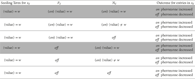
There is a caveat in this pheromone updating procedure given by the “ELSE IF” statement in Algorithm 2. It states that if P_d is off and the current particle and its best neighbour do not have the same seeding terms, then increase the likelihood of choosing the off state (by adding pheromone to the pheromone entry corresponding to the off value). The reason for this is to maintain the idea from the simple agent-based system described earlier in this section. That is, when two particles have different seeding terms, then those terms should tend to be omitted. Without this caveat the opposite would happen, the probability of the term being omitted would become less, as pheromone is usually removed from P_d (off) if P_d and N_d do not agree. A more detailed examination of the effect of the pheromone updating rules can be seen in Table 2 with this caveat being shown in the second row from the bottom.

Table 2. Different pheromone updating scenarios.

If after this process is completed any pheromone entry is less than a predefined minimum amount, then it is set to that amount (0.01). Importantly, this allows the pheromone entry that is not the best state to increase due to the normalisation procedure. This increase will occur if pheromone is removed from a state. If this happens, the amount of pheromone in the matrix becomes less than 1 and, as long as both entries have a greater than zero amount of pheromone, when the matrix is normalised both entries will increase. It also aids search in a conceptually similar way to mutation in GAs and the Min-Max system in the ACO literature [5].

In Table 2, the six possible scenarios for pheromone updating are described given the differing states of P_d, N_d and also the seeding term for x_d. These outcomes are controlled by the pheromone updating rules shown in Algorithm 2 (discussed previously). The first and last cases shown in the table are quite intuitive, if both P_d and N_d agree on a state that state is made more likely, this allows the algorithm to converge on a good solution that the particles agree on. Cases of the second type are shown in the second and fifth rows, where P_d and N_d have different seeding terms. In these cases, the particle makes it more likely that the conflicting term will be omitted from the decoded rule, by selecting the off state. This feature allows the particle to create rules that generalise well, covering more examples from the consequent class (discussed further in Section 3). Cases of the third type—which involve a disagreement between P_d and N_d about whether or not the seeded term should be used in the rule decoded from the current particle—are shown in the third and fourth rows. These cases bias the search towards N_d so that each particle tries to emulate its best neighbour. In the third row; if N_d = off then the probability of x_d decoding to off will be increased (by increasing the pheromone associated with the off state). In the fourth row; if N_d = w (and N_d and x_d have the same seeing terms) the probability of x_d decoding to on will be increased. The cases of the third type allow the particles to come to a consensus about the best set of states. By trying to emulate its best neighbour, each particle has the potential to create (in future iterations) a new past best state (P) based on a mix of its own current P and N.

2.3. A Differential Evolution Classification Algorithm for Continuous Data

Differential evolution (DE) [13] has become a popular optimisation algorithm for continuous spaces. It has been shown to be very competitive with respect to other search algorithms [18]. It can be considered a kind of evolutionary algorithm whose population moves around the search space in a greedy manner. Each offspring is (usually) generated from the weighted combination of the best member of the population with two or more other members of the population. If this offspring has a higher fitness then it replaces its parent, if not it is discarded. There are many variations on this basic evolutionary method for DE, the ones used in this paper are the rand-to-best/1 and best/1 as they seemed to be good during initial experiments. The formulas for offspring generation in these DE variants are as follows:

DE update equation for best/1:

()

DE update equation for rand-to-best/1

()

where v is the offspring vector, x_best is the best member of the current population. x_r1 and x_r2 are randomly-selected members of the population, x_i is the parent vector, and F is the weighting factor. The other parameters for the algorithm are: CR—a crossover likelihood factor and NP—the population size.

As we already have the framework for a PSO-based classification algorithm using sequential covering (as detailed in Section 2.1), the DE optimiser can essentially be “plugged-in,” replacing standard PSO as the rule discovery algorithm (for continuous data). To make any comparisons fair the same seeding mechanism and procedure to deal with crossed over attribute value bounds is used both in the PSO and DE classification algorithm.

2.4. Quality Measures

It is necessary to estimate the quality of every candidate rule (decoded particle). A measure must be used in the training phase in an attempt to estimate how well a rule will perform in the testing phase. Given such a measure, it becomes possible for an algorithm to optimise a rule′s quality (the fitness function). In our previous work [6], the quality measure used was Sensitivity × Specificity (9) [19].

Quality Measure used by PSO/ACO1 [6]:

()

where TP, FN, FP and TN are, respectively, the number of true positives, false negatives, false positives, and true negatives associated with the rule [1]:

(i)
true positives (TP) are the number of examples that match the rule antecedent (attribute values) and also match the rule consequent (class). These are desirable correct predictions;
(ii)
false positives (FP) are the number of examples that match the rule antecedent, but do not match the rule consequent. These are undesirable incorrect predictions;
(iii)
false negatives (FN) are the number of examples that do not match the rule antecedent but do match the rule consequent. These are undesirable uncovered cases and are caused by an overly specific rule;
(iv)
true negatives (TN) are the number of examples that do not match the rule antecedent and do not match the rule consequent. These are desirable and are caused by a rule’s antecedent being specific to its consequent class.

In the new PSO/ACO2 classification algorithm proposed in this paper, the quality measure is Precision with Laplace correction [1, 20], as per (10). In initial experiments this quality measure was observed to lead to the creation of rules that were more accurate (when compared to the original quality measure shown in (9).

New Quality Measure used by PSO/ACO2:

()

We observed that in some cases (when using (10) as a quality measure), rules would be generated covering very few examples. These cases were likely due to the way in which the Laplace-Corrected Precision measure penalises false positives very severely (when compared to Sensitivity × Specificity). To stop this less than ideal situation we added the following conditional statement to the new quality measure:

()

where MinTP is the least number of correctly covered examples that a rule has to cover before it is given a “normal” value, as computed by (10). When a rule covers too few examples the quality is severely reduced (by a factor of 100). This procedure reduces the quality below the quality of any normal rule, but still allows the particles covering fewer than MinTP examples to compare their solutions effectively. In our experiments, we set MinTP to 10, but any comparably small number will have a similar effect.

3. Motivations for PSO/ACO2 and Discussion

The modified algorithm (PSO/ACO2) proposed in this paper differs from the original algorithm (PSO/ACO1) proposed in [6, 7] in five important ways. Firstly, PSO/ACO1 attempted to optimise both the continuous and nominal attribute values present in a rule antecedent at the same time, whereas PSO/ACO2 takes the best nominal rule built by PSO/ACO2 and then attempts to add continuous attributes to it using a conventional PSO algorithm. Secondly, the original algorithm used a type of rule pruning to create seeding terms for each particle, whilst PSO/ACO2 uses all the terms from an entire training example (record). Thirdly, in PSO/ACO1 it was possible for a particle to select a value for an attribute that was not present in its seeding terms, whilst in PSO/ACO2 only the seeding term values may be added to the decoded rule. Fourthly, the pheromone updating rules have been simplified to concentrate on the optimisation properties of the original algorithm. In PSO/ACO1 pheromone was added to each entry that corresponded to the particle′s past best state, its best neighbour′s best state, and the particle′s current state in proportion to a random learning factor. Now, pheromone is only added to a pheromone matrix entry in the current particle when N_d and P_d match, or taken away when they do not. Fifthly, the algorithm now prunes the entire rule set after creation, not simply on a per rule basis.

In PSO/ACO2, the conventional PSO for continuous data and the hybrid PSO/ACO2 algorithm for nominal data have been separated partially because they differ quite largely in the time taken to reach peak fitness. It usually takes about 30 iterations (depending on the complexity of the dataset) for the pheromone matrices to reach a stable state in PSO/ACO2, whilst it tends to take considerably longer for the standard PSO algorithm to converge. Due to this fact, the standard PSO algorithm′s particles set past best positions in quite dissimilar positions, as their fitness is dependant on the quickly converging part of the PSO/ACO2 algorithm coping with nominal data. This causes high velocities and suboptimal search, with a higher likelihood of missing a position of high fitness. Therefore, separating the rule discovery process into two stages—one stage for the part of the PSO/ACO2 algorithm coping with nominal data and one stage for the part of the PSO/ACO2 algorithm coping with continuous data (essentially a variation of a standard PSO)—provides more consistent results.

Secondly, in the PSO/ACO1 algorithm, sets of seeding terms were pruned before they were used. This aggressive pruning algorithm used a heuristic to discard certain terms. This is less than ideal as the heuristic does not take into account attribute interaction, and so potentially useful terms are not investigated.

To understand the reasons behind the last two modifications, it is important to understand how the algorithms find good rules. In both PSO/ACO1 and PSO/ACO2, sets of terms are generated by mixing together the experiences of the particles and their neighbours. As the entries in the pheromone matrices converge and reach one (and zero), better rules should be generated more often. In PSO/ACO1, the levels of the pheromone in the matrices are influenced by three factors (current state, past best state, and best neighbours′ best state) [6]. If these factors do not agree, then the pheromone matrix will be slow to converge. Slow convergence can sometimes be advantageous as the algorithm should not prematurely converge to a local maximum. However, in PSO/ACO1 the result of this slow convergence is usually destructive, as incompatible terms can be mixed together over and over again. Incompatible terms are terms that do not cover any of the same examples. For instance, in Table 3, incompatible terms are A_n1 = a and A_n2 = b. A rule including both these terms would have a quality of zero as it would not cover any examples. This problem is addressed by the third modification in PSO/ACO2, now incompatible terms will not be mixed. This modification also ensures a particle will always cover at least one example (the seeding example) even if all the terms are included in the decoded rule. This was not the case in PSO/ACO1 as at the beginning of the search many incompatible terms could be mixed, creating many particles with zero fitness.

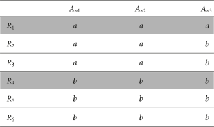Table 3. An example single class dataset, R′s are records, A_n′s are nominal attributes.

In PSO/ACO2, the pattern being investigated by the particles will likely include relatively general terms—an example might be a rule including the term A_n3 = b in Table 3. It is the job of the PSO/ACO2 algorithm to find terms that interact well to create a rule that is not only general to the class being predicted (covering many examples of that class) but also specific to the class (by not covering examples in other classes). It is also the job of the PSO/ACO2 algorithm to turn off terms that limit the generality of the rule without adding specificity to it. This trade-off between specificity and generality (or sensitivity) is calculated by the rule quality measure. It is clear, in Table 3, that including values for A_n1 and A_n2 will not ever lead to the most general rule (the optimal rule only has one term, A_n3 = b). Due to the new pheromone updating procedures a particle would choose the off state for these conflicting attributes quickly.

4. Results

For the experiments, we used 27 datasets from the well-known UCI dataset repository [21]. We performed 10-fold cross validation [1], and run each algorithm 10 times for each fold for the stochastic algorithms (PSO/ACO2 and the DE algorithm).

Both the part of the PSO/ACO2 algorithm coping with nominal data and the standard PSO algorithm (i.e., the part of PSO/ACO2 coping with continuous data) had 100 particles, and these two algorithms ran for a maximum of 100 iterations (MaxIterations) per rule discovered. In all experiments, constriction factor χ = 0.72984 and social and personal learning coefficients c1 = c2 = 2.05 [4]. PSO/ACO2 is freely available on sourceforge.

A freely available java implementation of DE by Mikal Keenan and Rainer Storn was used in all experiments presented in this paper [22]. The default values (as stated in the JavaDoc) of F = 0.5, CR = 1 for rand-to-best/1 and F = 0.5, CR = 1 for best/1 were used, so as not to delve into the realms of parameter tweaking. To maintain consistency with the PSO algorithm, a population size of 100 was used and the number of fitness evaluations was kept the same as the PSO variant. As to not bias the comparison, the PSO/ACO2 and DE classification algorithms were only compared on continuous attribute only datasets. This was done in an attempt to prevent any bias that might occur from the interaction with the nominal PSO/ACO2 part of the algorithm.

MaxUncovExampPerClass was set to 10 as this is standard in the literature [11]. As mentioned previously, PSO/ACO2 uses Von-Neumann topology, where each particle has four neighbours, with the population being connected together in a 2D grid. The corrected WEKA [1] statistics class was used to compute the standard deviation of the predictive accuracies and to apply the corresponding corrected two-tailed Student′s t-test—with a significance level of 5%—in the results presented in Tables 4, 5, and 6.

Table 4. Accuracy of labelled approaches in UCI datasets, with standard deviation and Student′s t-test shadings.

Table 5. Overall performance of PSO/ACO2 against PART according to WEKA’s Student′s t-test (out of 27 datasets).

	Accuracy	Average rule size	Average rule length
Total	1	−6	14

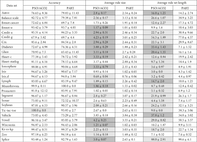
Table 6. Accuracy of labelled approaches in UCI datasets containing only continuous attributes, with standard deviation and Student′s t-test shadings.

The algorithms compared in Table 4 are PSO/ACO2 and PART. PART is WEKA’s improved implementation of C4.5 rules [1]. PART extracts rules from decision trees created by J48 (WEKA’s implementation of C4.5). We compared PSO/ACO2 against this algorithm as it is considered an industry standard.

The first two columns (not including the dataset column) in Table 4 show the percentage predictive accuracy of both algorithms. The second two columns show the average rule size (number of terms, or attribute-value pairs) for the rules generated for each dataset. The third two columns show the average rule set size for each dataset; this is simply the average number of rules in each rule set. The measures of average rule size and average rule set size give an indication of the complexity (and so comprehensibility) of the rule sets produced by each algorithm. The shading in these six columns denotes a statistically significant win or a loss (according to the corrected WEKA two-tailed Student′s t-test), light grey for a win and dark grey for a loss against the baseline algorithm (PART). Table 5 shows the overall score of the PSO/ACO2 classification algorithm against PART, considering that a significant win counts as “+1” and a significant loss counts as a “−1,” and then calculating the overall score across the 27 datasets.

It can be seen from Tables 4 and 5 that in terms of accuracy PART and PSO/ACO2 are quite closely matched. This is not completely surprising as PART is already considered to be very good in terms of predictive accuracy. Furthermore, there is only one result that is significant in terms of accuracy; the accuracy result for the tic-tac-toe dataset. However, if one scans through the accuracy results it is clear that often one algorithm outperforms the other slightly. In terms of rule set complexity, the algorithms are much less closely matched. When the average rule size results are taken as a whole, PSO/ACO2 generates longer rules in 6 cases overall. Although the average rule size results are significant, the real impact of having a rule that is under one term longer is arguable (as is found in many cases). The most significant results by far are in the rule set size columns. PSO/ACO produces significantly smaller rule sets in 14 cases overall, sometimes having tens of rules less than PART. These improvements have a tangible effect on the comprehensibility of the rule set as a whole.

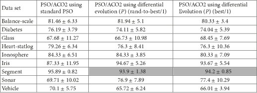
The reduced PSO/ACO2 classification algorithm (for continuous data only) using standard PSO (i.e., coping only with continuous attributes) is compared with the PSO/ACO2 classification algorithm using two DE variants in Table 6. Although there is one significant loss for each DE variant against the PSO variant, both algorithms seem to slightly outperform each other on certain datasets. Also, there is no clear winner between the different DE variants.

5. Discussion and Conclusions

We have conducted our experiments on 27 public domain “benchmark” datasets used in the classification literature, and we have shown that PSO/ACO2 is at least competitive with PART (an industry standard classification algorithm) in terms of accuracy, and that PSO/ACO2 often generates much simpler (smaller) rule sets. This is a desirable result in data mining—where the goal is to discover knowledge that is not only accurate but also comprehensible to the user.

At present, PSO/ACO2 is partly greedy in the sense that it builds each rule with the aim of optimising that rule′s quality individually, without directly taking into account the interaction with other rules. A less greedy, but possibly more computationally expensive way to approach the problem would be to associate a particle with an entire rule set and then to consider the quality of the entire rule set when evaluating a particle. This is known as the “Pittsburgh approach” in the evolutionary algorithm literature, and it could be an interesting research direction. Also the nominal part of the rule is always discovered first and separately from the continuous part, it could be advantageous to use a more “coevolved” approach.

Details are in the caption following the image — **Figure 1**
Open in figure viewer PowerPoint

The Von-Neumann topology used by PSO/ACO2.

References

1 Witten I. H. and Frank E., Data Mining: Practical Machine Learning Tools and Techniques, 2005, 2nd edition, Morgan Kaufmann, San Francisco, Calif, USA.
Google Scholar
2 Fayyad U. M., Piatetsky-Shapiro G., and Smyth P., From data mining to knowledge discovery: an overview, Advances in Knowledge Discovery and Data Mining, 1996, AAAI, Menlo Park, Calif, USA, 1–34.
Google Scholar
3 Kennedy J., Eberhart R. C., and Shi Y., Swarm Intelligence, 2001, Morgan Kaufmann/Academic Press, San Francisco, CA, USA.
Google Scholar
4 Bratton D. and [email protected], Kennedy J., [email protected], Defining a standard for particle swarm optimization, Proceedings of the IEEE Swarm Intelligence Symposium (SIS ′07), April 2007, Honolulu, Hawaii, USA, 120–127, https://doi.org/10.1109/SIS.2007.368035.
10.1109/SIS.2007.368035
Google Scholar
5 Dorigo M. and Stützle T., Ant Colony Optimization, 2004, The MIT Press, Cambridge, Mass, USA.
10.7551/mitpress/1290.001.0001
Web of Science® Google Scholar
6 Holden N. and [email protected], Freitas A. A., [email protected], A hybrid particle swarm/ant colony algorithm for the classification of hierarchical biological data, Proceedings of the IEEE Swarm Intelligence Symposium (SIS ′05), June 2005, Pasadena, Calif, USA, 100–107, https://doi.org/10.1109/SIS.2005.1501608.
10.1109/SIS.2005.1501608
Google Scholar
7 Holden N. and Freitas A. A., Hierarchical classification of G-protein-coupled receptors with a PSO/ACO algorithm, Proceedings of the IEEE Swarm Intelligence Symposium (SIS ′06), May 2006, Indianapolis, Ind, USA, 77–84.
Google Scholar
8 Sousa T., [email protected], Silva A., and [email protected], Neves A., [email protected], Particle swarm based data mining algorithms for classification tasks, Parallel Computing. (2004) 30, no. 5-6, 767–783, https://doi.org/10.1016/j.parco.2003.12.015.
10.1016/j.parco.2003.12.015
Web of Science® Google Scholar
9 De Falco I., [email protected], Della Cioppa A., and [email protected], Tarantino E., [email protected], Facing classification problems with particle swarm optimization, Applied Soft Computing. (2007) 7, no. 3, 652–658, https://doi.org/10.1016/j.asoc.2005.09.004.
10.1016/j.asoc.2005.09.004
Web of Science® Google Scholar
10 Freitas A. A., Parpinelli R. S., and Lopes H. S., M. Khosrou-Pour, Ant colony algorithms for data classification, Encyclopedia of Information Science and Technology, 2005, 2nd edition, IGI Publishing, Hershey, Pa, USA, 420–424.
Google Scholar
11 Parpinelli R. S., Lopes H. S., and Freitas A. A., Data mining with an ant colony optimization algorithm, IEEE Transactions on Evolutionary Computation. (2002) 6, no. 4, 321–332, https://doi.org/10.1109/TEVC.2002.802452.
10.1109/TEVC.2002.802452
Web of Science® Google Scholar
12 Dorigo M. and Socha K., T. F. Gonzalez, An introduction to ant colony optimization, Handbook of Approximation Algorithms and Metaheuristics, 2007, Chapman & Hall/CRC, Boca Raton, Fla, USA, 26.1–26.14.
10.1201/9781420010749.ch26
Google Scholar
13 Price K. V., Storn R. M., and Lampinen J. A., Differential Evolution: A Practical Approach to Global Optimization, 2005, Springer, Berlin, Germany.
Google Scholar
14 Holden N. and Freitas A. A., A hybrid PSO/ACO algorithm for classification, Proceedings of the 9th Genetic and Evolutionary Computation Conference Workshop on Particle Swarms: The Second Decade (GECCO ′07), July 2007, London, UK, ACM Press, 2745–2750, https://doi.org/10.1145/1274000.1274080.
10.1145/1274000.1274080
Google Scholar
15 Quinlan J. R., C4.5: Programs for Machine Learning, 1993, Morgan Kaufmann, San Francisco, Calif, USA.
Google Scholar
16 Pappa G. L., Automatically evolving rule induction algorithms with grammar-based genetic programming, Ph.D. thesis, Computing Laboratory, University of Kent, 2007, Canterbury, UK.
Google Scholar
17 Kennedy J. and Mendes R., Population structure and particle swarm performance, Proceedings of the IEEE Conference on Evolutionary Computation (CEC ′02), May 2002, Honolulu, Hawaii, USA, 1671–1676, https://doi.org/10.1109/CEC.2002.1004493.
10.1109/CEC.2002.1004493
Google Scholar
18 Mezura-Montes E., [email protected], Velázquez-Reyes J., and [email protected], Coello Coello C. A., [email protected], A comparative study of differential evolution variants for global optimization, 1, Proceedings of the 8th Annual Conference on Genetic and Evolutionary Computation (GECCO ′06), July 2006, Seattle, Wash, USA, ACM Press, 485–492, https://doi.org/10.1145/1143997.1144086.
10.1145/1143997.1144086
Google Scholar
19 Hand D. J., Construction and Assessment of Classification Rules, 1997, John Wiley & Sons, New York, NY, USA.
Google Scholar
20 Clark P. and Boswell R., Rule induction with CN2: some recent improvements, Proceedings of the 5th European Working Session on Learning (EWSL ′91), March 1991, Porto, Portugal, 151–163, https://doi.org/10.1007/BFb0017011.
10.1007/BFb0017011
Google Scholar
21 Newman D. J., Hettich S., Blake C. L., and Merz C. J., UCI repository of machine learning databases, 1998, http://www.ics.uci.edu/~mlearn/MLRepository.html.
Google Scholar
22 Differential Evolution Java Implementation, July 2007, http://www.icsi.berkeley.edu/~storn/code.html#java.
Google Scholar

Citing Literature

All articles

A Hybrid PSO/ACO Algorithm for Discovering Classification Rules in Data Mining

Abstract

1. Introduction

2. The New PSO/ACO2 Algorithm

2.1. PSO/ACO′s Sequential Covering Approach

2.2. The Part of the PSO/ACO2 Algorithm Coping with Nominal Data in Detail

2.3. A Differential Evolution Classification Algorithm for Continuous Data

2.4. Quality Measures

3. Motivations for PSO/ACO2 and Discussion

4. Results

5. Discussion and Conclusions

References

Citing Literature

Figures

References

Information

About Wiley Online Library

Help & Support

Opportunities

Connect with Wiley

A Hybrid PSO/ACO Algorithm for Discovering Classification Rules in Data Mining

Abstract

1. Introduction

2. The New PSO/ACO2 Algorithm

2.1. PSO/ACO′s Sequential Covering Approach

2.2. The Part of the PSO/ACO2 Algorithm Coping with Nominal Data in Detail

2.3. A Differential Evolution Classification Algorithm for Continuous Data

2.4. Quality Measures

3. Motivations for PSO/ACO2 and Discussion

4. Results

5. Discussion and Conclusions

References

Citing Literature

Figures

References

Related

Information