Coupling cellular automata and What If? models for residential expansion simulation: A case study of Southwest Sydney, Australia
Abstract
The impact of urban expansion on achieving sustainable development goals (SDGs) has become a significant research topic in the field of geographic information science. In this article, we describe a coupled cellular automata (CA)—-What If? model to explore SDG11 “Sustainable cities and communities.” The model calculates overall residential land use demand based on historical data archives using the What If? planning support system (PSS), and then allocates it using a CA model that incorporates variables related to SDG11.2.1 and 11.7.1. Historical datasets for years 2016 and 2021 from Southwest Sydney, Australia were used to assess model accuracy, after which two residential expansion scenarios (years 2021 and 2026) were generated. Based on the modeling results, the SDG-related spatial variables can improve the overall accuracy of CA sub-models using an XGBoost machine learning training methodology. The simulation results of these scenarios confirm the effectiveness of the coupled CA-What If? model, which has the potential to generate more reliable scenario results than the standalone What If? PSS for modeling urban growth of cities across Australia and internationally.
1 INTRODUCTION
The global population living in urban settlements reached 55% in 2018, and is projected to increase to 68% by mid-century (United Nations, 2018). This rapid urbanization presents both challenges and opportunities for policymakers and urban planners, who need to ensure there is sufficient housing stock and infrastructure facilities to accommodate the increasing population migrating to cities. With the expansion of metropolitan areas, the contrast between escalating demands for construction and the scarcity of available land resources becomes increasingly pronounced. Without robust urban planning instruments, rapid urban expansion can lead to a series of environmental issues, including air pollution (Hien et al., 2020), biodiversity decline (Huang et al., 2018), heat island effects (Zhu et al., 2020), and natural habitat loss (Tang et al., 2021). The increasing urbanization of the world's population has resulted in cities shouldering the responsibility to provide affordable housing resources to accommodate the influx of people (Han et al., 2021; Yates, 2016). However, significant carbon emissions are attributed to urban living, an issue that has raised the need for a “Net Zero” commitment (Hausfather & Moore, 2022). Likewise, many cities are experiencing increased traffic congestion and a declining quality of life for local residents (Truelove & Ruszczyk, 2022). In response to these issues, the United Nations has adopted the seventeen sustainable development goals (SDGs) (United Nations, 2016; Pizzi et al., 2020).
The latest version of the SDGs encompasses 169 specific goals and 231 indicators, establishing the sustainable development concept of “integrating economic development, social progress, and environmental improvement.” They require a holistic approach due to their complex, sometimes mutually reinforcing or conflicting nature, and achieving them demands methodical planning and action considering their interrelationships (Fu et al., 2019; Icsu, 2015). Since the inception of the SDGs, researchers have developed a range of urban simulation models incorporating SDGs-related variables or constraints, reflecting a growing interest in linking urban expansion and development with global sustainability goals (Cao, Tian, et al., 2023; Wang et al., 2021; Zhou et al., 2022). These models leverage geographic information systems (GIS), remote sensing, and machine learning techniques to simulate urban growth patterns, estimate future urban land use changes, and evaluate the implications on the SDGs.
Integrating SDG indicators into urban development strategies is an important approach for guiding cities toward enhanced sustainability and resilience. As urbanization accelerates, it becomes critically important to review our urban planning schemes and realign them to focus on SDGs, addressing a wide array of multifaceted challenges. For example, the conflict between urban expansion and agriculture highlights how economic policies can exacerbate poverty and environmental degradation (addressed in SDG 1) (Acheampong et al., 2018) and food production (addressed in SDG 2) (Barthel et al., 2019). This conflict underscores the need to control urban sprawl using certain rules. Furthermore, gender-responsive urban adaptation strategies (Susan Solomon et al., 2021) are closely related to sustainable urban planning and social–ecological–infrastructural systems of cities. Additionally, sustainable urbanization has been identified as a crucial component in the protection of intellectual property rights (Gao, Zhu, et al., 2022), and in assessing city metabolism (Musango et al., 2020), aligning with the framework of SDGs 9 and 11. In summary, there is a clear necessity for strategic and sustainable urban planning in line with specific SDGs, thereby fostering the development of sustainable and resilient cities at a global scale and address these challenges.
Among all goals, SDG 11 “Make cities and human settlements inclusive, safe, resilient, and sustainable” highlights the importance of solving key challenges of urban sustainability. With the ongoing trend of global urbanization, cities that adopt the SDG 11-related strategies are better positioned to balance a growing population by ensuring equitable access to both resources and infrastructure. Given the significance of SDG 11, specific targets under this goal have been applied in numerous urban modeling and analytical studies. Examples include access to housing (SDG 11.1) (Li, El-Askary, et al., 2020), access to transport (SDG 11.2) (Chen et al., 2019), and urban growth models for SDG 11.3 (Ghazaryan et al., 2021; Mithun et al., 2022). Key aspects of SDG 11.5, such as earthquakes (Takagi & Wada, 2019), flooding (Echendu, 2020), fire (Wei et al., 2021), and urban heat island changes (Meftahi et al., 2022; Zhu et al., 2020), have also been reported.
Cellular automata (CA) modeling is a well-established approach for modeling urban expansion and development (He et al., 2006; Lu et al., 2022a; Xu et al., 2019; Yang et al., 2023; Zhai et al., 2020). A classical CA model utilizes a lattice of equally sized cells, along with a set of attribute states to represent geographic features across urban spaces (Batty et al., 1999). By using state transition rules, the CA model can model changes in cell attributes at a micro-level, thereby collectively modeling the dynamic spatial–temporal evolution of the research area (Batty, 2009; Chen et al., 2014). This approach reflects the core concept of complexity science in that complex systems arise from the interaction of simple subsystems (Li, Yeh, et al., 2020). Many aspects of CA models have been explored, including cell forms (Liang et al., 2021; Lu et al., 2015; Yang et al., 2023; Zhu et al., 2021), the discovery of transition rules (Cao et al., 2019; Ding et al., 2022; Momeni & Antipova, 2020), delimitation of neighbourhoods (Barreira-González & Barros, 2017; Zhai et al., 2021), as well as constraint and parameter sensitivity (Li et al., 2021; Wu et al., 2019; Yang et al., 2022).
Some researchers have experimented with integrating SDG indicators and CA modeling. For instance, the CA-Markov model, a commonly used modeling framework, integrates economy (SDG2.3.1 and SDG8.1.1), social (SDG3.c.1, SDG4.1.2, SDG5.b.1, SDG9.c.1, SDG 9.1.2, SDG11.2.1, and SDG11.7.1) and environmental (SDG6.3.1 and SDG11.6.2) related SDG indicators as variables for land use prediction, spatial allocation, and as evaluation metrics (SDG11.3.1) for land use efficiency. Operating through macro-level Markov processes and micro-level CA-based simulation, these models have been applied in the Niger Delta region (Musa et al., 2019), Yangtze River Delta region (Cao et al., 2022), and Tianjin metropolitan area (Lu, Qureshi, et al., 2022). These coupled SDG-Markov-CA models have been demonstrated to provide a comprehensive framework for achieving specific targets in simulating urban expansion and development processes. However, the integration of SDG indicators with the CA models is still underexplored, as evidenced by the limited number of case studies.
CA models enable an understanding of urban expansion and simulation of development. Nevertheless, accurate projections of urban land patterns also require established scenarios that represent possible future socioeconomic and environmental characteristics (Chen et al., 2020; Debnath, Pettit, Soundararaj, et al., 2023). The What If? planning support system (PSS) is a bottom-up model, featuring standalone suitability evaluation, demand projection, and spatial allocation functions. It is a scenario-based tool that uses GIS data for land suitability analysis, land use projection, and evaluation of policy impacts on urban development (Klosterman, 1999, 2011; Pettit et al., 2015). In this research, a CA model is integrated with the What If? PSS to identify future urban development patterns more comprehensively and reliably across a set of scenarios.
The article is divided into five sections. Following this introduction, the fundamental structure, components, and methodologies of the model. Subsequently, a detailed case study from the Southwest of the Greater Sydney Region, Australia is given in Section 3. The simulation results and predicted scenarios are then analyzed in Section 4, while Section 5 provides a summary of key findings and outlines future research directions.
2 METHODOLOGY
2.1 The general CA-What If? modeling framework
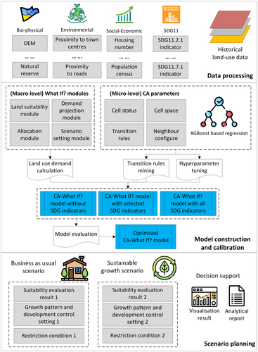
The general CA-What If? modeling framework can be divided into three key stages (Figure 1). The first stage involves input data, which comprises historical land use change maps and spatial variables, including biophysical, environmental, socioeconomic, and SDG-related indicators. Socioeconomic-related variables, such as historical population, the number of dwellings, vacancy rate, and average household size, are utilized for land use demand projection at the macro level. The biophysical, environmental, and SDG-related spatial variables, associated with land use change maps serve as the driving factors of land use change at the macro level. The processed land use datasets are then randomly selected as separate training and testing samples. In the second stage, the What If? demand sub-model derives past trends in housing supply and population growth, and then projects future land use demand. Simultaneously, key parameters of the CA sub-model are fine-tuned via hyperparameter adjustments employing a decision tree-based regression methodology. This process is pivotal for discovering the transition rules of the CA sub-model. Afterward, the CA sub-model integrates typical spatial variables and SDG-related indicators to assess whether the inclusion of SDG indicators enhances the overall performance of land use allocation. Quantitative evaluation and validation, including the use of producer's spatial accuracy metrics and kappa coefficients, are integral to the model validation process. In the third stage, the optimized CA-What If? framework is then utilized to simulate future land use scenarios, applying various strategies and growth patterns to further analyze the model's outputs. The final outputs are the land use change layouts under each of the potential scenario, and are then further evaluated and visualized for decision-making support.
2.2 Land use demand calculation using What If?
2.3 CA model calibration using XGBoost
3 CASE STUDY
3.1 Study area and data processing
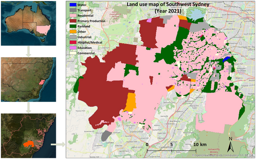
Southwest Sydney is located within the Greater Sydney region in Australia, featuring Cabramatta and Liverpool as two of its key urban centers. The bounding polygon used here is the “Sydney–South West” Statistical Area Level 4, as defined by the Australian Statistical Geography Standard (ABS, 2021b), with an area of 540.42 km2. In the most recent population census, the region accommodated 155,782 private dwellings (households), and a total population of 474,430 (ABS, 2021a). In terms of population growth, it is one of the fastest-growing regions in Australia, reflecting the continued immigration trend seen throughout the Greater Sydney region, with consistently high demand for residential properties (Lu et al., 2023). The official projection from the NSW Planning Institute indicates that the population of the entire Greater Sydney region is expected to surpass 6.1 million by 2041, an increase of over 1 million people from the current population (NSW Government, 2022). Moreover, the predominant land use change within Southwest Sydney is toward newly developed residential areas (Figure 2). With an increasing population and evident trend in residential development, Southwest Sydney has been identified as an ideal place for the verification of the proposed CA-What If? modeling framework.
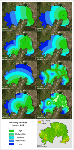
- Proximity (Figure 3a–h). Proximity variables measure accessibility and are commonly employed in land use change modeling. Proximity in this study is measured as the Euclidean distances from the Sydney CBD (DCBD), the town center of Southwest Sydney (DCen), shopping centers (DShop), public hospitals (DHosp), universities (DUni), main roads (DRoad), train stations (DRail), and parklands (DPark). The latter two variables serve as localised indicators of SDG 11.2.1 and SDG 11.7.1, relating to public space accessibility for all, inclusive of gender, age, and persons with disabilities.
- Slope (Figure 3i). The topographical slope gradient significantly influences the feasibility and cost of building construction. The slope of the study area was calculated using a 1-second Digital Elevation Model (DEM) provided by Geoscience Australia (2011), which has been processed to represent ground surface topography. The highest slope values are in the western and southern parts of the study area, reaching a maximum of 40.6°.
- Constraint. Any land use transformation is excluded within listed reserve areas as outlined in Table 1.
| Variable name | Definition | Data source |
|---|---|---|
| D CBD | Distance to the Sydney CBD | OpenStreetMap |
| D cen | Distance to the town center of Southwest Sydney | OpenStreetMap |
| D Shop | Distance to the nearest shopping center | OpenStreetMap |
| D Hosp | Distance to the nearest public hospital | OpenStreetMap |
| D Uni | Distance to the Western Sydney University—Liverpool Campus | OpenStreetMap |
| D Road | Distance to the nearest main roads | Geoscience Australia |
| Slope | The slope of the candidate cell | Geoscience Australia |
| LimitReserve | Spatial information on areas reserved under the NP&W Act 1974. Areas include National Parks, Nature Reserves, Regional Parks, State Conservation Areas, Aboriginal Areas, Historic Sites and Karst Conservation Reserves | NSW Government—The NSW National Parks and Wildlife Service (NPWS) Estate database |
| DRail (SDG11.2.1-related) | Distance to the nearest railway stations within Southwest Sydney | Geoscape Australia |
| DPark (SDG11.7.1-related) | Distance to the nearest parkland | Australian Bureau of Statistics |
- Note: All the spatial variables (except for LimitReserve) have been normalized to the value range of [0, 1] to exclude the impacts of differentiated units.
In the simulation experiments, all CA sub-models utilized a 3 × 3 Moore Neighbourhood configuration, comprising a total of 100 iterations per experiment. A random disturbance variable (Equation 5) was used to simulate stochastic perturbations.
The data processing workflow comprises several distinct stages. First, land use categories are derived from the ABS Mesh Block polygons for Southwest Sydney between 2016 and 2021, and then converted to raster with a resolution of 60 × 60 m. Cells that changed the category to “Residential” land use between these two time periods were identified, with most changed cells initially being “Primary Production,” “Parkland,” and “Other.” The required variables for calculating the overall demand (Equations 1-3) were then input into the ‘What If?’ sub-model to estimate residential demand for 2026. Subsequently, the spatial variables are then spatially joined with the candidate raster cells, namely those categorized as “Primary Production,” “Parkland,” and “Other.” The values of these spatial fields are either the Euclidean distance from a candidate cell to the nearest POIs and FOIs, the slope of candidate cells, or whether a candidate cell is situated within the reserve areas (LimitReserve). Given the dataset size (66,356 records) and the incorporation cross-validation during the hyperparameter tuning process, the entire dataset has been randomly divided into training (30%) and testing (70%) samples. These samples were used for hyperparameter tuning to optimize the performance of the XGBoost-based CA sub-model. Upon deriving the optimal parameter combination, four groups of XGBoost-CA sub-models with different sets of spatial variables were developed to assess the impact of SDG-related variables in spatial allocation.
3.2 The land use demand of Southwest Sydney
Future residential-related land use demand was modeled using historical census data (ABS, 2021a). The population, number of dwellings, vacancy rates, and average household sizes were derived directly from the ABS census data for the years 2016 and 2021 (ABS, 2016, 2021a). The density of residential housing was estimated by dividing the number of dwellings by the total area of the Sydney Southwest polygons (Table 2).
| Year | Population | Number of dwellings | Vacancy rate (%) | Average household size (persons/household) | Density of residential housing (houses/km2) |
|---|---|---|---|---|---|
| 2016 (actual) | 405,962 | 122,954 | 4.9 | 3.3 | 239.75 |
| 2021 (actual) | 474,430 | 148,543 | 5.6 | 3.2 | 288.34 |
| 2026 (predicted) | 503,607 | Not required | 4.9 | 3.3 | 295.10 |
The projected population of the entire Greater Sydney region at the commencement of years 2021 and 2026 are 5,259,800 and 5,583,600, respectively (Australian Government, 2023). Given this growth rate of 6.15%, the predicted population of Southwest Sydney is 503,607 and the predicted density of residential housing is 306.07.
| Land use category | Year 2016 | Year 2021 | ||
|---|---|---|---|---|
| Area (km2) | Fraction (%) | Area (km2) | Fraction (%) | |
| Commercial | 3.70 | 0.68 | 4.99 | 0.92 |
| Education | 5.33 | 0.99 | 6.04 | 1.12 |
| Hospital/medical | 0.30 | 0.06 | 0.30 | 0.06 |
| Industrial | 18.39 | 3.40 | 18.36 | 3.40 |
| Other | 13.20 | 2.44 | 10.18 | 1.88 |
| Parkland | 66.89 | 12.38 | 63.89 | 11.82 |
| Primary Production | 158.79 | 29.38 | 144.33 | 26.71 |
| Residential | 272.38 | 50.40 | 287.97 | 53.29 |
| Transport | 0.70 | 0.13 | 3.61 | 0.67 |
| Water | 0.74 | 0.14 | 0.74 | 0.13 |
| Total | 540.42 | 100.00 | 540.42 | 100.00 |
3.3 Hyperparameter tuning
The parameters of XGBoost algorithm were refined using random search coupled with a stratified threefold cross-validation approach (‘GridSearchCV’ function in the scikit-learn Python library, version 1.4), for hyperparameter tuning purpose (Pedregosa et al., 2011). Hyperparameter tuning was conducted to enhance the XGBoost regressor's capability in predicting whether a candidate cell has been transferred to “Residential” at the end of the simulation period. Explanatory variables were “DCBD,” “DCen,” “DShop,” “DHosp,” “DUni,” “DRoad,” “DRail,” “DPark,” “Slope,” (Table 1) and “Neighbourhood”. The hyperparameters identified as most effective, as detailed in Table 4, were then used to configure an enhanced XGBoost regressor model. [Correction added on 23 July 2024, after first online publication: The Explanatory variable `Neighbourhood’ added after first online publication.]
| Hyperparameter | Definition | Values tested | Optimal parameter |
|---|---|---|---|
| n_estimator | Number of gradient-boosted trees | 100, 200, 300 | 300 |
| learning_rate | Learning rate | 0.01, 0.1, 0.2 | 0.1 |
| max_depth | Maximum depth of a tree | 3, 4, 5 | 5 |
| min_child_weight | Minimum sum of instance weight needed in a child | 1, 2, 3 | 1 |
| subsample | Subsample ratio of the training instances | 0.6, 0.8, 1.0 | 0.8 |
| colsample_bytree | The fraction of features to be randomly sampled for each tree | 0.6, 0.8, 1.0 | 0.8 |
3.4 XGBoost-based CA sub-model training and testing
After hyperparameter tuning, four groups of spatial variables were applied to CA sub-models 1–4 for training purposes. CA sub-model 1 utilized all variables, including those related to both SDG11.2.1 (DRail) and SDG11.7.1 (DPark). CA sub-models 2 and 3 each utilized all variables except for DRail and DPark, respectively. CA sub-model 4 was trained exclusively with non-SDG-related variables. Additionally, each CA sub-model was trained and tested through 10 independent simulations, and the simulation process for each single CA sub-model consists of 100 iterations. Each simulation iteration can be simplified into three steps: (1) Calculate the transfer probabilities of all candidate cells; (2) Select cells with higher transfer potentials for conversion based on their overall probabilities in the current iteration; (3) Update the selected candidate cells to residential cells and update the spatial layers accordingly. After 100 iterations, the simulated distribution of residential and nonresidential cells for the year 2021 is produced for each of the CA sub-models. Finally, the 2016 testing sample is utilized as the reference for model evaluation.
An evaluation of four CA sub-models, highlighting the substantial influence of incorporating SDG-related variables (specifically DRail and DPark) is given in Table 5. Specifically, producer's spatial accuracy and kappa coefficients are being applied as the metrics for CA sub-model evaluation. Sub-model 1, which includes all variables, demonstrates superior accuracy, achieving producer's spatial accuracy scores ranging from 96.50% to 97.52%, with a mean of 97.14%. Its average kappa coefficient of 0.967 also exceeds that of the other groups. This enhanced spatial accuracy and consistency underscores the effectiveness of integrating SDG-related variables. [Correction added on 23 July 2024, after first online publication: The spacial accuracy scores 97.14% corrected to 96.50% and 96.50% corrected to 97.14%.]
| Variable | Producer's spatial accuracy | Kappa coefficient | |||||
|---|---|---|---|---|---|---|---|
| Max (%) | Min (%) | Mean (%) | Max | Min | Mean | ||
| Sub-model 1 | DCBD, Dcen, DShop, DHosp, DUni, DRoad, DRail, DPark, Slope, Neighbourhood | 97.52 | 96.50 | 97.14 | 0.971 | 0.959 | 0.967 |
| Sub-model 2 | DCBD, Dcen, DShop, DHosp, DUni, DRoad, DRail, Slope, Neighbourhood | 97.13 | 96.24 | 96.59 | 0.967 | 0.956 | 0.960 |
| Sub-model 3 | DCBD, Dcen, DShop, DHosp, DUni, DRoad, DPark, Slope, Neighbourhood | 97.46 | 96.37 | 96.87 | 0.971 | 0.958 | 0.964 |
| Sub-model 4 | DCBD, Dcen, DShop, DHosp, DUni, DRoad, Slope, Neighbourhood | 96.31 | 92.87 | 95.49 | 0.957 | 0.917 | 0.948 |
The DUni variable appears to be the most significant variable across all sub-models (Table 6). The SDG11.7.1-related variable, DPark, is also important, particularly in sub-models 1 and 3 for which it records values of 14.0% and 16.2%, ranking as the second highest in feature importance among all variables. The DCBD variable is identified as the third-highest in feature importance across all models except for sub-model 2. Additionally, the SDG 11.2.1-related variable DRail demonstrates feature importance values of 7.8% and 11.0%, ranking 5th and 4th highest in sub-models 1 and 2, respectively. These findings affirm the pivotal impact of specific SDG-related variables on the simulation accuracy of the model. [Correction added on 23 July 2024, after first online publication: The sentence `The DCBD variable is identified as the third-highest in feature importance across all models’ corrected to `The DCBD variable is identified as the third-highest in feature importance across all models except for sub-model 2’]
| Variable name | Average feature importance (%) | |||
|---|---|---|---|---|
| Sub-model 1 | Sub-model 2 | Sub-model 3 | Sub-model 4 | |
| D CBD | 12.4 (3) | 13.6 (2) | 12.5 (3) | 13.2 (3) |
| D cen | 6.5 (6) | 8.2 (5) | 8.8 (5) | 13.2 (3) |
| D Shop | 5.9 (8) | 7.8 (6) | 7.6 (6) | 8.0 (5) |
| D Hosp | 8.6 (4) | 11.8 (3) | 9.9 (4) | 16.6 (2) |
| D Uni | 33.1 (1) | 34.2 (1) | 33.3 (1) | 31.0 (1) |
| D Road | 6.4 (7) | 7.0 (7) | 5.9 (7) | 6.8 (7) |
| DRail (SDG11.2.1 related) | 7.8 (5) | 11.0 (4) | n.a. | n.a. |
| DPark (SDG11.7.1 related) | 14.0 (2) | n.a. | 16.2 (2) | n.a. |
| Slope | 1.2 (10) | 3.2 (8) | 2.6 (9) | 5.2 (8) |
| Neighbourhood | 4.0 (9) | 3.1 (9) | 3.2 (8) | 6.9 (6) |
- Note: The average feature importance is calculated based on the mean value of 10 separate operations of each type of CA sub-model, the numbers in the brackets indicate the relative importance of these features in sub-models.
3.5 Scenario planning outcomes using a CA-What If? model
The importance of SDG-related variables in CA sub-modeling has been shown in the preceding section. Consequently, CA sub-model 1, which uses all spatial variables listed in Table 6, is selected for allocating the overall land use demand from the What If? sub-model.
Scenario planning was initially introduced by Royal Dutch/Shell in the late 1960s to early 1970s for generating and evaluating strategic options (Wack, 1985). As awareness of urban growth and sustainable development grew, scenario planning began to be applied for forecasting and analyzing urban land use changes (Chakraborty & McMillan, 2015; Pettit et al., 2020; Wang et al., 2022). Figure 4 illustrates the spatial distribution of newly developed residential land under two scenarios: “Business as Usual” and “Sustainable growth.” Additionally, Table 7 shows the proportions of newly transformed residential cells in every SA3. In the “Business as usual” scenario, the transformation rules and the types of land eligible for a from 2016 to 2021. Here, newly added residential cells for 2021–2026 area selected from the “Primary Production,” “Parkland” and “Other” categories. In contrast, the “Sustainable growth” scenario, while maintaining the identical transition rules for land use demand allocation, reduces the types of available categories to “Primary Production” and “Other.”
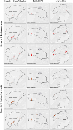
Scenario modelling results by the CA-What If? model for Southwest Sydney, Australia.
Note: The red areas represent newly developed residential land after specific iterations under the proposed scenarios. [Correction added on 23 July 2024, after first online publication: Figure 4 is replaced, the text in figure `Scenario 2:Eco-freindly’ corrected to `Scenario 2: Sustainable growth’.]
| SA3 name | Scenario 1. Business as usual | Scenario 2. Sustainable growth | ||
|---|---|---|---|---|
| Number of new residential cells | Proportion (%) | Number of new residential cells | Proportion (%) | |
| Bringelly—Green Valley | 1015 | 60.49 | 1260 | 75.09 |
| Fairfield | 162 | 9.65 | 257 | 15.32 |
| Liverpool | 501 | 29.86 | 161 | 9.59 |
To evaluate the accuracy of future land use predictions, three spatial layers are used: biodiversity value, bushfire-prone areas, and proposed future residential growth areas (Table 8). The actual future land use is obviously unknown, making a calculation of the overall accuracy or Figure of Merit (FoM) in the traditional sense infeasible.
| Name | Description | Data source and year | Link |
|---|---|---|---|
| Biodiversity Values Map | The Biodiversity Values Map (BV Map) identifies land with high biodiversity value that is particularly sensitive to impacts from development and clearing. The BV Map is one of the triggers for determining whether the Biodiversity Offset Scheme (BOS) applies to a clearing or development proposal | NSW Government (2018) | https://datasets.seed.nsw.gov.au/dataset/biodiversity-values-map |
| NSW Bushfire-Prone Land | Bushfire-Prone Land is mapped within a local government area, which becomes the trigger for planning for bushfire protection. Bushfire-Prone Land mapping is intended to designate areas of the State that are considered to be higher bushfire risk for development control purposes | NSW Government (2020) | https://datasets.seed.nsw.gov.au/dataset/bush-fire-prone-land |
| Growth centers | The proposed areas of growth centers outlined in in State Environmental Planning Policy (Precincts–Western Parkland City) | NSW Government (2021) | https://prod.planning-nsw.links.com.au/opendata/dataset/state-environmental-planning-policy-precincts-western-parkland-city-2021 |
4 DISCUSSION
Between 2016 and 2021, the overall proportion of “Residential” land in the study area increased from 50.40% to 53.29%, with an associated decrease in “Primary Production,” “Parkland,” and “Other” categories. This reflects a general trend of urban residential expansion in order to satisfy population growth and related housing demand in the entire Greater Sydney region over the past decades. It corresponds to the latest version of the Greater Sydney region Plan (NSW Government, 2018), which anticipates an increased demand and preference for housing to meet the needs of evolving communities. Thus, it can be inferred that the conversion of nonresidential to residential land is likely to remain the dominant land use trend in the Greater Sydney region for the upcoming future.
To explore and simulate the spatial distribution of prospective land use change in the uncertain future, this article proposes a coupled CA-What If? modeling framework which simulates urban residential expansion under various scenarios. The What If? sub-model predicts the overall land demand in the study area between 2021 and 2026 at a macro-level scale, drawing on the historical Australian national census data (years 2016 and 2021), along with the manual setting of the vacancy rate, average household size and density of residential housing in the year 2026 by taking past trend as reference. It is suggested by this forecast that from 2021 to 2026, an additional of 6.04 km2 residential land will be required in Southwest Sydney, in comparison with the previous 15.59 km2 change of residential land from 2016 to 2021. This trend suggests changes in the compact city form and increasing densification of Southwest Sydney, characterized by smaller land parcels for single detached housing alongside a rise in apartments and higher density developments (Easthope et al., 2022; Kleeman et al., 2022).
Regarding our CA sub-model, the effectiveness of two SDG-related spatial variables is validated in terms of their impacts on the spatial allocation accuracy. Afterward, the CA sub-model with selected spatial variables, which generate the most accurate outcome, is used for future scenario planning. Different combinations of spatial variables affect the CA sub-models' accuracy (Table 5), even in a relatively small area like Southwest Sydney. Incorporating two SDG-related variables resulted in an average producer's accuracy of 97.14% from 10 independent simulations, higher than when only a single SDG factor was considered (96.59% and 96.87%). The sub-model without SDG factors had the lowest spatial allocation accuracy, ranging between 92.87% and 96.31%. Furthermore, the importance of the SDG-related variables was also evident in the spatial rule extraction results based on the XGBoost method. The spatial variable DPark (Related to SDG 10.7.1) ranked second in feature importance in both sub-models 1 and 3, while DRail (Related to SDG 11.2.1) ranked fifth and fourth in sub-models 1 and 2, respectively (Table 6). These findings underscore the significance of SDG spatial variable in the overall accuracy of CA sub-models.
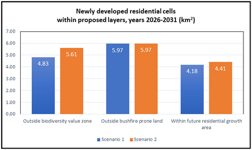
After fine-tuning and validation, the CA sub-model is then applied for the allocation of the overall land use demand for Southwest Sydney, with 100-iteratons in each of the proposed simulation experiments. Scenario 2 “Sustainable growth” better integrates natural risk management with urban development planning than Scenario 1 “Business as usual” (Figure 5). Specifically, there is a total of 5.61 km2 newly transformed residential cells outside biodiversity value zones in Scenario 2, compared with 4.83 km2 cells in Scenario 1. This enhancement signifies a more ecologically considerate approach to urban residential expansion, aiming to minimize impacts on biodiversity value. In addition, there is also a slight rise in the number of cells within proposed growth centers in Scenario 2 (4.41 km2) compared with Scenario 1 (4.18 km2), reflecting a targeted commitment to development within planned growth boundaries. Moreover, the identical figures for newly transformed cells outside bushfire-prone land (5.97 km2 in both Scenarios 1 and 2) demonstrate a consistent emphasis on preventing bushfire risks while balancing developmental ambitions. These evaluation standards from Figure 5 prove that Scenario 2 has advanced the reconciliation of State Environmental Planning Policy (Precincts—Western Parkland City) in our case study. It is also concluded that in comparison with large-scale urban land expansion scenarios (Chen et al., 2020), even within a relatively short simulation period (5 years) and a relatively small study area (540.42 km2), small adjustment of land use conversion rules in proposed scenarios can lead to significant differences in the simulation results of the study area. These findings are also consistent with previous CA model or What If?-based scenario planning (Daniel & Pettit, 2022; Debnath, Pettit, & Leao, 2023; Feng et al., 2019; Liang et al., 2018).
5 CONCLUSIONS
This research represents an exploration of integrating CA and What If? models, where the What If? sub-model is utilized for land use demand prediction, and the CA sub-model is used to allocate overall demand to specific raster cells. Specifically, the What If? sub-model predicts that the conversion from nonresidential to residential land will continue as the primary trend in urban development in Southwest Sydney. Less newly developed residential land is expected between 2021 and 2026 (6.04 km2) compared with the period 2016–2021 (15.59 km2). In comparison with its initial version (Lu et al., 2022b), the CA sub-model in this study is calibrated using the XGBoost machine learning algorithm, is capable of discerning complex and nonlinear landscape change patterns in this region, a finding echoed by other researchers in similar studies in Khulna city, Bangladesh (Islam et al., 2021), Yancheng City, China (Hao et al., 2022), Seoul, Korea (Kim et al., 2023), separately. In conclusion, the modeling outcome reveals that Scenario 2 ‘Sustainable Growth’ is more effective in balancing residential expansion needs with reduced bushfire risk compared with Scenario 1 “Business as Usual.” Furthermore, it aligns more closely with the growth centers proposed by the NSW Department of Planning.
Overall, the coupled CA-What If? model is not only capable of capturing the regulations of historical urban residential expansion and SDG-related indicators, but also to predicting the future residential land use demands at a macro-level, and then allocating these demands at a micro-level. However, there is still potential for further improvement in its framework. For instance, further categorizing residential land into types, such as low, medium, and high-density, corresponding to diverse housing types, could enhance the framework's realism, particularly with regard to cell types in the CA sub-model. Furthermore, the What If? sub-model could consider both constraints on land transformation and land use change priority in specific areas, as demonstrated for a different region by Pettit et al. (2015). It could also incorporate the synergies and trade-offs among complex SDG indicators, which is crucial to achieving long-term sustainability goals (Cao, Chen, et al., 2023; Hegre et al., 2020; Kuc-Czarnecka et al., 2023). Finally, validating the coupled CA-What If? model's applicability in larger metropolitan areas, such as the entire Greater Sydney or other metropolitan regions would be the next step in testing the generality of the model. This would assess the impact of spatial heterogeneity rules on the model's performance across different subregions in a further step.
ACKNOWLEDGMENTS
This research was enabled through the Australia Research Data Commons (ARDC) and Australian Urban Research Infrastructure Network (AURIN) funded – Australian Housing Data Analytics Platform (RG203395). The authors are also grateful for the data provided by the Australian Bureau of Statistics (ABS) and OpenStreetMap (OSM). Open access publishing facilitated by University of New South Wales, as part of the Wiley - University of New South Wales agreement via the Council of Australian University Librarians.
CONFLICT OF INTEREST STATEMENT
The authors declare no potential conflicts of interest with respect to the research, authorship, and publication of this paper.
Open Research
DATA AVAILABILITY STATEMENT
The ABS Mesh Block polygon dataset used in this study is available at https://www.abs.gov.au/statistics/standards/australian-statistical-geography-standard-asgs-edition-3/jul2021-jun2026/access-and-downloads/digital-boundary-files.


