A decade of photo-identification reveals contrasting abundance and trends of Type B killer whales in the coastal waters of the Antarctic Peninsula
Funding information: E. R. Johnson; Lindblad Expeditions- National Geographic Conservation Fund, Grant/Award Numbers: LX07-15, LX07-16, LX07-17, LX07R-18; National Oceanic and Atmospheric Administration; Pew Charitable Trusts, Grant/Award Number: 32659; SR3
Abstract
The Antarctic Peninsula (AP) is rapidly warming and empirical data on abundance trends of marine organisms are required to understand the impact of these physical changes, and interacting anthropogenic impacts, on the ecosystem. Recent estimates inferred increasing abundance of Type A killer whales at the top of this food chain, and here we provide new data on the abundance of Type B1 and B2 killer whales using photographic mark-recaptures collected during austral summers from 2008/2009 to 2017/2018. Both ecotypes were regularly photographed around the AP coastline, particularly off the west side, and individuals of both showed site fidelity across years. B1s had a higher re-identification rate (58% photographed in multiple years, range: 1–7 years) compared to B2s (31%, 1–4 years). We fit mark-recapture models that allowed temporary emigration beyond the study area, to effectively monitor the size of wide-ranging populations and documented contrasting trends for B1s and B2s. A smaller population size (~102) of B1s was estimated to use the area, with a declining trend in abundance (−4.7% per year) and reduced apparent survival in recent years. In contrast, a much larger population size (~740) of B2s was estimated to be generally stable in abundance and apparent survival over the past decade.
1 INTRODUCTION
The Antarctic Peninsula (AP) is one of the most rapidly warming regions on the planet (Li, 2014; Meredith & King, 2005; Mulvaney et al., 2012; Siegert et al., 2019; Turner & Comiso, 2017; Vaughan et al., 2001, 2003). Additionally, there are increasing anthropogenic impacts, for example rapidly proliferating shipping traffic from ecotourism, and these may interact with environmental changes (Convey & Peck, 2019). As such, empirical data on abundance and trends of marine predator and prey populations are required to understand the impact of these physical changes on the trophic dynamics of this ecosystem (Cimino et al., 2019; Convey & Peck, 2019; Peck et al., 2004).
There is increasing recognition of the ecosystem importance of apex predators (Estes et al., 2011), including killer whales (Orcinus orca) in Antarctic waters (e.g., Ainley et al., 2010). Around the AP, killer whales are represented by three phenotypically, genetically, and culturally distinct ecotypes (Types B1, B2, and A; Durban et al., 2017; Fearnbach et al., 2019; Foote et al., 2011, 2013, 2016; LeDuc et al., 2008; Morin et al., 2010, 2015; Pitman & Durban, 2010, 2012; Pitman & Ensor, 2003). Recent estimates have inferred increasing abundance of Type A killer whales (Fearnbach et al., 2019), an open-water, mammal-eating form that is more typical in appearance to killer whales sighted in other parts of the world. In contrast, there are currently no data on the abundance or trends of Antarctic Type B killer whales. Two forms of Type B killer whales have been described (Durban et al., 2017; see Figure 1), both sharing the distinctive dorsal cape pigmentation and large postocular eye patches: a larger, more pagophilic mammal-eating form (B1) that specializes on hunting ice seals on pack ice floes (Pitman & Durban, 2012) and a smaller, gregarious more open water form (B2) that has to date been reported to feed on pygoscelid penguins (Pitman & Durban, 2010), and Weddell seals (Leptonychotes weddellii; Pitman, Durban & Fearnbach, unpublished data), and regularly dives to depths between 500 m and 700 m, suggesting a principal diet of fish or squid (Pitman et al., 2020). Type B killer whales are neritic in occurrence, typically occurring in the shallow waters of the continental shelf (Pitman & Ensor, 2003), are rarely observed away from Antarctica, and show evidence of physiological adaptations to living in these frigid waters (Foote et al., 2011, 2016). Although, they make periodic migrations to warm subtropical waters, they return rapidly to feed in the coastal waters off the AP (Durban & Pitman, 2012; Pitman et al., 2020).
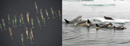
Evaluation of the trophic impact of Type B killer whales around the AP requires information on their population abundance and trends at appropriate spatial scales for ecosystem considerations. Individual killer whales can be identified by distinctive and long-lasting natural markings, and photographs of individuals can be used to construct identification histories (e.g., Balcomb et al., 1982; Bigg, 1982; Bigg et al., 1990; Ford et al., 2000). This photo-identification approach has been successfully applied to provide robust population assessments in readily accessible populations that can be monitored through complete annual photographic censuses (Bigg et al., 1990; Ford et al., 2000; Matkin et al., 1999, 2008). However, killer whales in more remote environments, which are both costly and challenging to survey, require a mark-recapture sampling approach for abundance estimates (e.g., Durban et al., 2010; Pitman et al., 2018; Fearnbach et al., 2019). We applied a Bayesian mark-recapture approach to 10 years of photo-identification data to estimate abundance and evaluate the population status of Type B1 and B2 killer whales around the AP. Our findings fill key data gaps about these important apex predators in this rapidly changing marine ecosystem.
2 METHODS
2.1 Photo-identification data
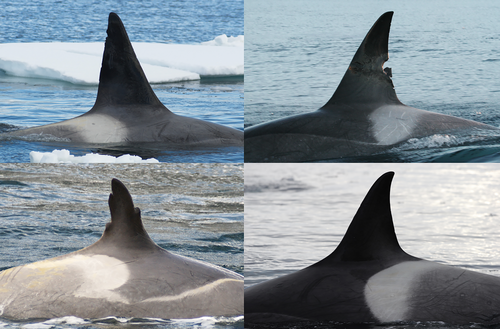
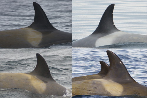
Photo-identification images were collected in the austral summers between 2008/2009 and 2017/2018 from a variety of platforms, including tourism expedition ships and research vessels. These images were collected opportunistically by the authors and by contributors from other vessels. Digital images were used to identify as many individual whales as possible based on distinctive dorsal fin profiles (e.g., nicks and shape), saddle patch pigmentation, and scarring patterns (Figures 2 and 3). The best right and/or left image of each individual in each group encounter was compared to an existing photo-identification catalog. If a match was found, the individual was assigned the existing identification number, and if no match was found, the individual was assigned a new identification number and added to the catalog. Mark-recapture analysis requires that individuals have natural markings that are distinctive enough to allow for repeat identifications over time. Therefore, each image was graded for quality and distinctiveness following Durban et al. (2010). Quality grades indicated which part of the individual was captured in the image and whether the image was usable for analyses, based on focus, angle, and clarity due to image exposure. An image was assigned a grade of 4 when it showed a usable dorsal fin and saddle, a 3 for a usable fin only, a 2 for a usable saddle only, and a 1 for a poor-quality image. Distinctiveness scores were assigned for each individual and were based on a presence or absence of identifying marks that were divided into six categories: distinctive dorsal fin shape, nicks in the dorsal fin, distinctive saddle pigmentation pattern, black scratches on the saddle, white scratches on the saddle, and oval scars on the saddle caused by cookie-cutter sharks, Isistius spp. These features have been shown to be retained on individual Antarctic killer whales for at least 14 years (Pitman et al., 2018). An individual was included in analyses if it possessed at least two distinctive marks that were visible on the body feature that was documented in useable quality.
2.2 Mark-recapture model
To estimate the number of whales using the study area, but not always present, we fit mark-recapture models that allowed for temporary emigration beyond the bounds of the study area (Fearnbach et al., 2019; Matkin et al., 2012; Whitehead, 1990). This may have occurred as a result of whale movement, but also likely reflected interannual changes in the effective area that could be accessed by ships and resultant changes in the availability of whales for sampling. In particular, annual differences in ice cover resulted in portions of the study area being inaccessible to vessel traffic in some years, and therefore time-varying population coverage was assumed. These effects can be included in mark-recapture models by including terms for the transition of individuals to and from an unobservable state, but identification of these parameters requires model constraints, notably imposing temporal constancy of parameters (Kendall & Nichols, 2002). We therefore chose to model the identification probability of whales in the effective study area as constant across years, in order that key variability in whale availability was captured in a time-varying formulation. However, we also compared the fit of models with time-varying identification probability, constant availability, and no temporary emigration (see below).
The model describes change on the log scale and therefore β represented the rate of change in population size across years, and was assigned a noninformative Uniform distribution. The base population size, μP, was assigned a U(min[Ot], 2000) prior with the lower boundary set as the minimum number of distinctive whales that were actually observed in any year.
We used the NIMBLE package to fit the model within the R statistical environment. Inference was based on Markov Chain Monte Carlo sampling for 50,000 iterations after discarding an initial burn-in of 50,000 iterations. Summary statistics for the posterior distributions were then estimated from the sampled values. To assess the evidence that the rate of population change parameter, β, differed from zero (no change), we monitored the proportion of the post burn-in MCMC values for which the parameter value was above or below zero (Gerrodette, 2011).
As with other model selection methods, the predictive criterion achieves a compromise between the goodness-of-fit and a penalty for the number of free parameters in the model (Gelfand & Ghosh, 1998). The model with the smallest criterion value was estimated to be the model that would best predict a replicate data set of the same structure as that currently observed.
The predictive model selection criterion does not necessarily reveal whether a selected model is a plausible fit for the observed data. We therefore also adopted a posterior predictive approach for goodness-of-fit checking for the best-fit model (Durban et al., 2010; Gelman et al., 1996). A discrepancy measure, D, was calculated for both the simulated Xnew and observed data X as the sum of the absolute differences between observed identification histories and binary predictions from the parameters of the mark-recapture model (described by Durban & Elston, 2005). The discrepancy measures themselves had posterior distributions, and so they could be compared by estimating the exceeding tail area probability as the percentage of MCMC draws for which D(Xnew) > D(X). The result is a Bayesian (or posterior predictive) p-value: values close to .5 indicate that the simulated discrepancy of the data is similar to what is expected from replication under the model. If the model is a poor fit to the data, the Bayesian p-value will be close to 0 or 1 (Gelman et al., 1996).
3 RESULTS
3.1 Photo-identification samples
3.1.1 Type B1 photo-identifications
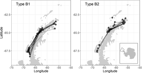
A total of 9,847 photographs were taken during 79 encounters with Type B1 killer whales in AP coastal waters (Figure 4). We identified 2,518 best whale-by-encounter images, of which 2,115 were judged to be useable quality. From these, we identified 123 distinctive fins from both left and right-side photographs. Extensive photographic re-identifications were made across the study area, between the far western Weddell Sea in the north and the southern end of Adelaide Island in the south (Figure 4). We therefore focused abundance analysis on images from all 79 encounters located within a polygon 60.5°–69°S, 50°–70°W collected during 10 consecutive austral summers from 2008/2009 to 2017/2018 (Table 1). We were able to identify 107 distinctive individuals from left-side photographs and 107 from right sides. We based identification histories only on right-side photographs because there were more whale-by-year records, but used left-side matches of these whales to input data on annual availability and survival status.
| Year | Date range | Encounters | Photographs | Whales |
|---|---|---|---|---|
| 2008–2009 | Nov 24–Feb 27 | 22 | 6,180 | 37 |
| 2009–2010 | Oct 12–Jun 5 | 9 | 424 | 40 |
| 2010–2011 | Nov 27–Jan 24 | 7 | 155 | 19 |
| 2011–2012 | Nov–Feb 23 | 3 | 166 | 13 |
| 2012–2013 | Dec 12–Mar 4 | 7 | 1,255 | 28 |
| 2013–2014 | Nov 15–Jan 22 | 7 | 462 | 36 |
| 2014–2015 | Nov 25–Feb 8 | 9 | 84 | 19 |
| 2015–2016 | Nov 22–Jan 14 | 7 | 116 | 23 |
| 2016–2017 | Nov 1–Feb 10 | 3 | 640 | 11 |
| 2017–2018 | Nov 24–Mar 3 | 5 | 365 | 22 |
The right-side data consisted of 248 positive records in the binary whale-by-year identifications of these 107 whales. The number of whales identified from right-side images varied each year, ranging from 11 to 40; individuals were identified during 1–7 different years (median of 2 years) and 62 whales (58%) were identified in >1 year. With the inclusion of left-side identifications of these same whales, an additional 57 records were added, generating 305 positive records in the binary whale-by-year availability matrix. We added 102 further positive records to survival status for imputation between years with repeat sightings. When we considered the range of years between first and last sightings, almost half (51 individuals) were known to be alive across at least half the time series (5 or more years), and 11 whales were known from all 10 years.
3.1.2 Type B2 photo-identifications
A total of 25,117 photographs were taken during 63 encounters with Type B2 killer whales in AP waters (Figure 4). We identified 2,908 best whale-by-encounter images, of which 2,779 were judged to be useable quality. From these, we identified 704 distinctive fins from both left and right-side photographs. Photographic re-identifications were made across the study area from the far western Weddell Sea in the north to Adelaide Island in the south, but identifications (and re-identifications) were concentrated in the Gerlache Strait area off the central western AP (Figure 4). As such, we focused abundance analysis on images collected coastally within a polygon 60.5°S–69°S, 50°W–70°W collected during 10 consecutive austral summers from 2008–2009 to 2017–2018 (Table 2). We identified 575 distinctive individuals from left-side photographs and 567 from right-sides. We based identification histories only on left-side photographs because there were more whale-by-year records, but used right-side matches of these whales to input data on annual availability and survival status.
| Year | Date range | Encounters | photographs | Whales |
|---|---|---|---|---|
| 2008–2009 | Jan 8–Jan 28 | 7 | 2,821 | 106 |
| 2009–2010 | Feb 13–Feb 28 | 7 | 2,877 | 97 |
| 2010–2011 | Jan 15–Feb 4 | 3 | 156 | 46 |
| 2011–2012 | Jan 10–Feb 13 | 6 | 4,142 | 114 |
| 2012–2013 | Jan 11–Feb 18 | 5 | 1,026 | 44 |
| 2013–2014 | Dec 2–Feb 11 | 8 | 2,599 | 100 |
| 2014–2015 | Dec 13–Feb 12 | 6 | 519 | 86 |
| 2015–2016 | Jan 12–Feb 23 | 7 | 3,062 | 74 |
| 2016–2017 | Dec 24–Feb 3 | 6 | 2,248 | 103 |
| 2017–2018 | Nov 23–Feb 12 | 8 | 5,667 | 78 |
The left-side data consisted of 848 positive whale-by-year binary identifications for the 575 distinctive whales. The number of whales identified from left-side images varied each year, ranging from 46 to 114 (Table 2). Individuals were identified during 1–4 different years (median of 1 year), but 181 whales (31%) were identified in >1 year. When we imputed right-side identifications of these same whales, we added 95 positive records for a total of 943 positive records in the binary whale-by-year availability matrix. We added a further 548 positive records to the survival status for imputation between years with repeat sightings. When we considered the range of years between first and last sightings, 109 individuals (19%) were known to be alive across at least half the time series (five or more years), and 26 whales were known from all 10 years.
3.2 Mark-recapture model
Model selection supported the full model with time-varying parameters for survival and availability, with a constant identification probability for whales that were in the study area (Table 3). Notably, this model predicted a new data set displaying closer agreement to the observed identification histories than the five other plausible models, with 171 predicted errors over the 1,070 binary observations for B1s and 453 errors over 5,750 observations for B2s (Table 3). Further inference was therefore based solely on this model, which also provided an adequate fit to the data, with Bayesian p-values of .51 for B1s and 0.52 for B2s, indicating that the data were similar to expected replications under the model (Gelman et al., 1996).
| Predicted error | ||
|---|---|---|
| Model | Type B1 | Type B2 |
| π ϕt εt λt | 171 | 453 |
| π ϕ εt λt | 184 | 466 |
| πt ϕt ε λ | 181 | 468 |
| πt ϕ ε λ | 189 | 475 |
| πt ϕt | 181 | 468 |
| πt ϕ | 189 | 482 |
Both populations were readily monitored using natural markings, with an estimated 85% and 95% of the individuals having distinctive marks for B1s and B2s, respectively. Mark-recapture coverage was much higher for B1s than B2s, with mean identification probabilities of 0.38 and 0.16, respectively (Table 4). There were notable changes in availability between years for both B1s and B2s, with a median annual probability of transitioning from available to unavailable of 0.20 for B1s (range of annual posterior median estimates = 0.03–0.57) and 0.16 for B2s (range = 0.03–0.65) (Table 4). Individuals in both populations had a relatively high rate of transitioning from unavailable to available, with a median probability of 0.56 for B1s (range = 0.14–0.90) and 0.69 for B2s (range = 0.34–0.89), indicating our ability to rediscover and track the population despite availability gaps in identification histories (Table 4). Type B2s typically had a higher annual rate of apparent survival, with a median of annual estimates of 0.96 compared to 0.93 for B1s (Table 4). Type B1s were estimated to have recent reductions in survival: the median annual survival rate over the first 5 years (2009–2014) was 0.95, compared to only 0.88 over the last 4 years. In contrast, annual apparent survival estimates of B2s were more consistent at a median of 0.95 over the first 5 years and 0.96 over the recent 4 years. However, there was one anomalously low survival estimate for B2s between 2016 and 2017 of 0.81, representing the lowest survival for any year for either type.
| Parameter | Type B1 | Type B2 |
|---|---|---|
| Identification probability (π) | 0.38 (0.31, 0.46) | 0.16 (0.14, 0.19) |
| Survival probability (ϕ) | 0.93 (0.88, 0.98) | 0.96 (0.81, 0.98) |
| Available to NA probability (ε) | 0.20 (0.03, 0.57) | 0.16 (0.03, 0.65) |
| NA to available probability (λ) | 0.56 (0.14, 0.90) | 0.69 (0.34, 0.89) |
| Average population (μP) | 102 (77–138) | 740 (556–1,183) |
| Annual rate of abundance change (β) | −0.047 (−0.13, 0.04) | 0.003 (−0.09, 0.11) |
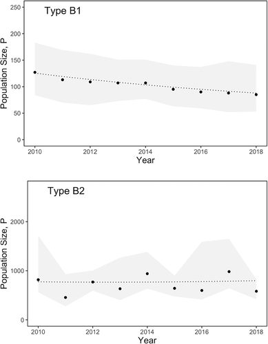
After accounting for distinctiveness and availability, population estimates showed contrasting trends for the two types. Annual population estimates for B1s ranged from 77 to 138, with an estimated declining trend of −4.7% a year (Figure 5). The posterior distribution for the annual rate of population change mostly fell below zero, with a high probability (p = .84) that the B1 population has been generally decreasing over the last decade. Annual population estimates for B2s ranged from 556 to 1,183, with the posterior distribution for the annual rate of population change falling almost symmetrically around zero, indicating a generally stable population over the last decade, with very little support (p = .52) for population increase or decrease (p = .48).
4 DISCUSSION
This study provides the first data on the abundance and trends of two forms of Type B killer whales in the coastal waters of the AP. Using photo-identification matches, we identified a coastal area off the AP where both Type B1 and B2 killer whales were consistently encountered and photographed. There were notable hot spots off the western AP for both types: for B2 killer whales in the Gerlache Strait area and for B1s between Adelaide Island and mainland AP. Both types were also encountered off the northern tip of the AP in the far western Weddell Sea. We used a Bayesian mark-recapture approach to analyze and communicate uncertainty about population parameters using full probability distributions (Durban et al., 2000; Gelman et al., 1995). This method has been shown to be useful for making inference on population dynamics within open and wide-ranging populations of cetaceans where uncertainty arises from more opportunistic sampling designs (Durban et al., 2010; Fearnbach et al., 2012). Despite reported “skin-molt migrations” away from Antarctica (Durban & Pitman, 2012; Pitman et al., 2020), we documented repeated use of the study area by many of the same whales for both types across years, although the rate of re-identification was higher for Type B1s. Individual whales of both types were identified across a large area that was likely surveyed to different extents across years. Despite this, we rediscovered individuals across years and parameterized our mark-recapture models with availability terms to effectively monitor the size of the population using the area, even if some of these whales were not in the effective study area to be sampled in some years.
We estimated a much higher average population size of B2 killer whales (~740) compared to B1s (~102), although considerable turnover for both forms implied that not all of the population was available to be photographed in each year. Contrasting trends in abundance were estimated over the 10-year sampling period, with the population estimates of B1s declining at a rate of −4.7% per year, with notably lower survival during the latter part of the study. In contrast, B2s were generally stable in abundance, with consistently higher survival estimates. However, anomalously low annual survival towards the end of the study for B2s highlighted a potential change in population dynamics and the importance of continued monitoring to build on this time series.
Although there was overlap in the distribution of both types, B1s were generally encountered closer to shore and had a more southerly skew to encounter locations. This indicated their affinity for areas with a greater chance of retaining pack ice in the austral summer, where they can locate their preferred ice-seal prey, notably Weddell seals (Pitman & Durban, 2012). This key foraging habitat is becoming scarce in the summer as sea ice declines around the AP; this may explain the population declines of B1 killer whales, but we cannot currently differentiate between demographic changes and possible redistribution that influenced apparent survival. The comparatively high and stable abundance of Type B2 killer whales is likely a response to a locally abundant prey (e.g., Gentoo penguins; Bestelmeyer et al., 2011; Cimino et al., 2016) and access to available ice-free foraging habitat where they are typically encountered undertaking prolonged feeding bouts characterized by deep diving (Pitman et al., 2020). The target species of this deep foraging and the proportion of this prey item in their diet, remains a key data gap for understanding their future population dynamics and vulnerability to the changing environment (see Lee et al., 2017; Turner & Comiso, 2017).
A number of low and mid-level consumer populations have already been shown to be impacted by the rapidly changing physical environment and resulting ecosystem changes around the AP (Bestelmeyer et al., 2011; Cimino et al., 2016, 2019; Peck et al., 2004). In combination with Fearnbach et al. (2019), which found an increase in the abundance of Type A killer whales in the western AP between 2005 and 2017, this study suggests population impacts on the top predators. Specifically, the killer whales that prefer open water habitats (Type B2s and As) appear to be stable and benefitting, respectively, from the loss of sea ice and subsequent increase in available open water foraging habitat, while the pagophilic Type B1 killer whales may be struggling with declines in sea-ice and subsequent habitat loss for their primary prey of ice seals. Such a pattern parallels observed population trends for penguins off the western AP, where ice-obligate Adélie penguins (Pygoscelis adeliae) have been declining and ice-intolerant Gentoo penguins (Pygoscelis papua) have been increasing in recent decades (Bestelmeyer et al., 2011).
ACKNOWLEDGMENTS
This paper would not have been possible without the contribution of photographs from many dedicated naturalists and photographers, and we are grateful to IAATO for promoting our project and encouraging photographic submissions. We were ably assisted in the field by Lindblad Expedition staff, crew, and officers onboard the National Geographic Explorer. We are also very grateful to Simon Morley and colleagues from the British Antarctic Survey's Rothera Research Station for their contribution of photographs. The authors also collected photo-identification images from platforms of opportunity provided by the BBC and the US Antarctic Program. Photo-identification analysis was supported by the Pew Charitable Trusts, the Lindblad Expeditions-National Geographic Conservation Fund and a private grant from E. R. Johnson. Field research by the authors was conducted under Antarctic Conservation Act Permits 2009-013 and 2017-29 issued by the U.S. National Science Foundation, and Marine Mammal Protection Act Permits 774-1714 and 19091 issued by the U.S. National Marine Fisheries Service. We also thank George Watters and Dave Weller for commenting on an earlier version of this manuscript.
AUTHOR CONTRIBUTIONS
Holly Fearnbach: Conceptualization; data curation; formal analysis; funding acquisition; investigation; methodology; project administration; resources; software; supervision; validation; visualization; writing-original draft; writing-review & editing. John Durban: Conceptualization; data curation; formal analysis; funding acquisition; investigation; methodology; project administration; resources; software; supervision; validation; visualization; writing-original draft; writing-review & editing. David Ellifrit: Formal analysis. Alyssa Paredes: Formal analysis. Leigh Hickmott: Investigation; writing-review & editing. Robert Pitman: Conceptualization; funding acquisition; investigation; resources; writing-review & editing.


