The score-driven approach to time series modelling is able to handle circular data and switching regimes with intra-regime dynamics. Furthermore it enables a dynamic model to be fitted to a linear and a circular variable when their joint distribution is a cylinder. The viability of the new method is illustrated by estimating models for hourly data on wind direction and speed in Galicia, north-west Spain. The modelling of intra-regime dynamics is shown to be of critical importance.

1 INTRODUCTION

Many areas of environmental statistics involve applications where circular data are collected and statistically analysed. For example, modelling and forecasting wind direction is relevant for tracking pollution and wildfires. Harvey et al. (2022) show how a score-driven approach1provides a solution to time series modelling of circular data. The present article extends this approach to handle data from time series where there is switching between different regimes and shows how dynamic bivariate models for speed and direction can be constructed.

The viability and effectiveness of the new methods is illustrated with data on wind direction and speed at a wind farm site in Galicia, North-West Spain. The observations were taken every minute over the month of January 2004. These data are used by García-Portugués et al. (2013) in a study of pollution. Figure 1 shows the time series of observations, measured in radians from 0 to $2 π,$ obtained by taking the last observation in each hour. Zero radians corresponds to due east with the subsequent coding being anti-clockwise so $π / 2$ is north, $π$ is west and $3 π / 2$ is south. Because of circularity some of the measurements in the North East (NE) orbit appear at the top, close to $2 π,$ rather than near the bottom. Serious distortions can arise if circularity is not taken into account and standard linear time series methods are used.

Details are in the caption following the image — **Figure 1**
Open in figure viewer PowerPoint

Hourly wind direction and speed in January 2004 at a site in Galicia

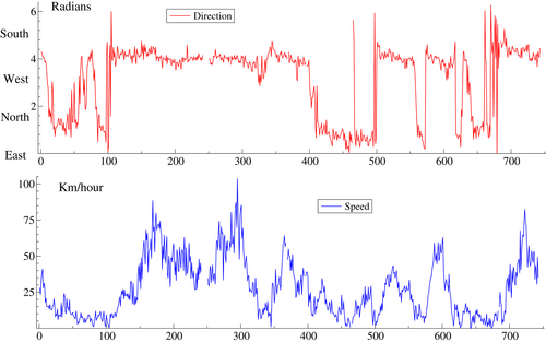
García-Portugués et al. (2013) note that the prevailing wind comes from two directions: SW and NE. The two dominant directions are apparent in Figure 1 with NE being a little less than one radian and SW around four. Hence a regime switching model may be appropriate. Holtzmann et al. (2006) propose a switching regime model for wind direction and the same approach is used by Zucchini et al. (2016, pp. 228–35), for modeling the change in direction of flight for fruit flies. The basic formulation assumes a finite number of regimes and introduces dynamics by a Markov chain in which there is a fixed probability of staying in the current regime or moving to another; see Hamilton (1989, 1994). The regime is not observed: hence the term hidden Markov model (HMM) as in Zucchini et al. (2016). The probability of being in a particular regime is given by a filter that depends on past observations. These probabilities yield a conditional mixture distribution for the current observation and hence a likelihood function. Catania (2021) proposes a different approach that by-passes the hidden Markov chain and instead sets up filters for the regime probabilities in the conditional distribution directly by using their scores. He calls these dynamic adaptive mixture models (DAMMs). The score-driven approach leads naturally to a solution of how to model intra-regime dynamics. The key point is that the forcing variables in dynamic equations are a function of past observations weighted according to the probability that they are in a given regime. Intra-day dynamics have not been modelled in this way in standard HMMs. Yet in many environmental applications there are marked intra-regime dynamics. The evidence presented here shows that neglecting these dynamics can be a major drawback.

Figure 1 also shows wind speed. Wind speed is a (non-negative) linear variable and a joint model distribution of a linear and a circular variable takes the form of a cylinder. Abe and Ley (2017) proposes a general distribution for cylindrical data. A key feature of their distribution is that the circular concentration is allowed to increase with the linear component, a phenomenon first identified in the seminal article by Fisher and Lee (1992, p. 666). The challenge is to move from the static to the dynamic case. We show here that a score-driven approach facilitates the construction of a model that allows the location of the circular variable and the level (scale) of the linear variable to change over time. The concentration may also change.

The bivariate score-driven model can be incorporated in a regime switching model. Switching bivariate models have been used by Lagona et al. (2015) for modeling the joint distribution of wave height and direction in the Adriatic; they employ an HMM for fitting a cylindrical distribution when there are three distinct regimes. Other applications involving speed and direction include tracking and forecasting the movements of animals, boats and wildfires, as in García-Portugués et al. (2014).

Section 2 reviews the score-driven model for circular data proposed by Harvey et al. (2022) and fits it to wind direction in Galicia. The theory underlying regime switching models is described in section 3 and it is shown how the score-driven approach set out in Section 2 is able to model dynamic location and concentration within regimes. The methods are applied to the Galicia data on wind direction in Section 4. Dynamic cylindrical distributions are described in Section 5 and extended to handle switching regimes. These time series models are fitted to the Galicia data on direction and speed in Section 6. Section 7 concludes.

2 SCORE-DRIVEN MODELS FOR CIRCULAR DATA

Circular observations measured in radians are usually taken to have a von Mises (vM) distribution with probability density function (PDF)

f (y; μ, υ) = \frac{1}{2 π I_{0} (υ)} \exp {υ \cos (y - μ)}, - π \leq y, μ < π, υ \geq 0,

(1)

where

I_{k} (υ)

denotes a modified Bessel function of order

k

μ

is mean direction and

υ

is a non-negative concentration parameter that is inversely related to dispersion. When

υ = 0

the distribution is uniform whereas

y

is approximately

N (μ, 1 / υ)

for large

υ .

The maximum likelihood (ML) estimator of location,

μ,

is the sample mean direction,

{\overline{y}}_{d};

see Mardia and Jupp (2000). A class of general circular distributions, in which the cardioid and wrapped Cauchy are special cases, is described in Jones and Pewsey (2005).

Circular time series models currently in use are almost all based on the autoregressive-moving average (ARMA) type models proposed in Fisher and Lee (1994) or are regime switching models; see Pewsey and García-Portugués (2021, section 10.1). Score-driven models offer considerable advantages and allow regime switching to be combined with intra-regime dynamics.

2.1 Dynamic Location

Data generated by a time series model over the real line, that is

- \infty < z_{t} < \infty,

can be converted into wrapped circular time series observations in the range

[- π, π)

by letting

y_{t} = z_{t} mod (2 π) - π, t = 1, \dots, T;

(2)

see Breckling (1989) and Fisher and Lee (1994). The score-driven model for circular data is

z_{t} = μ_{t | t - 1} + ε_{t}, - π \leq ε_{t} < π, t = 1, \dots ., T,

(3)

where the

ε_{t}^{'} s

are independent and identically distributed (IID) random variables from a circular distribution with location zero and

μ_{t | t - 1}

is a filter for location at time

t

based on information available at time

t - 1

. The basic stationary first-order filter is

μ_{t + 1 | t} = (1 - ϕ) ω + ϕ μ_{t | t - 1} + κ u_{t}, |ϕ| < 1, t = 1, \dots, T,

(4)

where

μ_{1 | 0} = ω

is the unconditional location of

μ_{t | t - 1}

and the forcing variable,

u_{t},

is defined as being (proportional to) the conditional score for location, that is

\partial \ln f (y_{t}; μ_{t | t - 1}, υ) / \partial μ_{t | t - 1}, t = 1, \dots, T

A defining property of a (continuous) circular distribution is that it satisfies the periodicity condition $f (z \pm 2 π k; ψ) = f (z; ψ),$ where $k$ is an integer and $ψ$ denotes parameters. Provided the derivatives of the log-density with respect to the elements of $ψ$ are continuous, they too are circular in that the periodicity condition is satisfied. Thus the path of $μ_{t | t - 1}$ is the same irrespective of whether $u_{t}$ is defined in terms of $z_{t}$ or $y_{t} .$ The conditional distribution of $y_{t}$ in a model defined by (3), (4) and (2) is therefore the same as that of $z_{t}$ and so the likelihood function of the wrapped observations, the $y_{t}^{'} s,$ is the same as that of the unobserved variables, the $z_{t}^{'} s$ .

In the case of the von Mises distribution, that is

ε_{t} \sim v M (0, υ)

in (3), the score is

u_{t} = υ \sin (z_{t} - μ_{t | t - 1}) = υ \sin (y_{t} - μ_{t | t - 1}), u_{t} ∽ I I D (0, A (υ) / υ) .

(5)

The general continuous circular distribution of Jones and Pewsey (2005) has a score that, like (5), is invariant to wrapping as well as being IID.

Harvey et al. (2022) provide further details and derive the asymptotic distribution of the ML estimators of $ϕ,$ $κ$ and $ω$ in (4) for the stationary vM model.

2.2 Tests

The Lagrange multiplier, or score, test against serial correlation in location is based on the portmanteau or Box–Ljung statistic constructed from the autocorrelations of the scores; see Harvey (2013, section 2.5). For a vM distribution with $υ > 0$ , the scores under the null hypothesis of constant location are proportional to $\sin (y_{t} - {\overline{y}}_{d}) .$ Hence the sample autocorrelations correspond to the circular autocorrelations (CACFs) in Jammalamadaka and SenGupta (2001, pp. 176–9).

2.3 Heteroscedasticity

Score-driven models can be extended to allow for dynamic heteroscedasticity by setting up a filter for the conditional concentration. Thus

ε_{t}

in (3) is distributed as

v M (0, υ_{t | t - 1})

with the dynamics dependent on the score with respect to

υ_{t | t - 1}

, that is

u_{t}^{υ} = \cos (y_{t} - μ_{t | t - 1}) - A (υ_{t | t - 1}) .

The scores are a martingale difference sequence with mean zero and variance

1 - A {(υ_{t | t - 1})}^{2} - A (υ_{t | t - 1}) / υ_{t | t - 1} .

An exponential link function can be used to ensure the concentration remains positive. Thus

υ_{t | t - 1} = \exp (ζ_{t | t - 1}) .

The first-order dynamic model for

ζ_{t | t - 1}

is then

ζ_{t + 1 | t} = (1 - ϕ_{ζ}) ω_{ζ} + ϕ ζ_{t | t - 1} + κ u_{t}^{ζ}, t = 1, \dots, T,

(6)

where

u_{t}^{ζ} = υ_{t | t - 1} u_{t}^{υ}

and

ζ_{1 | 0} = ω_{ζ} .

The likelihood function is

\ln L (ψ) = - T \ln (2 π I_{0} (υ_{t | t - 1})) + \sum_{t = 1}^{T} υ_{t | t - 1} \cos (y_{t} - μ_{t | t - 1}),

where

ψ

denotes the parameters in the dynamic equations for

υ_{t | t - 1}

as well as

μ_{t | t - 1} .

The forcing variable for location is now

u_{t} = υ_{t | t - 1} \sin (y_{t} - μ_{t | t - 1})

2.4 Application to Circular Data from Galicia

When a basic first-order dynamic model, (4) is fitted to the Galicia data,2 the result is $\tilde{ϕ} = 1.0,$ $\tilde{κ} = 0.19$ and $\tilde{υ} = \exp ({\tilde{ω}}_{ζ}) = 4.78 .$ The maximized log-likelihood is $\ln L = - 510.62$ . The residual CACF shows there is considerable serial correlation remaining and the fit, as measured by dispersion (circular variance), is no better than that of a random walk in which $μ_{t | t - 1} = y_{t - 1};$ see Mardia and Jupp (2000, pp. 18–19 and 30). Adding heteroscedasticity gives a better fit, but although this reduces the serial correlation in dispersion, the serial correlation in location increases.

3 SWITCHING REGIMES

The plot of wind direction in Galicia provides a clear motivation for a switching model. The first subsection below gives a short description of the static mixture model before moving on to review the dynamic adaptive mixture model (DAMM) of Catania (2021). The third subsection then shows how the score-driven approach can handle intra-regime dynamics and in the subsection following the associated diagnostic tests are set out. The last subsection discusses circular observations.

3.1 Static Mixture Model

The PDF of a mixture of

K

distributions is

f (y_{t}; ψ) = \sum_{i = 1}^{K} ξ_{i} f_{i} (y_{t}; ψ_{i}), \sum_{i = 1}^{K} ξ_{i} = 1, t = 1, \dots, T,

where

0 \leq ξ_{i} \leq 1

i = 1, 2, \dots, K,

with

ξ_{i},

denoting the probability of being in

i

th regime; the parameters in the

i

th regime are contained in the vector

ψ_{i}

and

ψ

includes all these parameters, together with

ξ_{i}, i = 1, 2, \dots, K - 1

. When the observations are independent, the probability of being in regime

i

given observation

y_{t}

ξ_{i} (y_{t}) = ξ_{i} f_{i} (y_{t}; ψ_{i}) / f (y_{t}; ψ), i = 1, 2, \dots . K .

(7)

The maximum likelihood (ML) estimates for the parameters in each of the $ψ_{i}^{'} s,$ together with the unconditional probabilities, $ξ_{i},$ $i = 1, \dots, K,$ can be computed iteratively by what turns out to be a special case of the EM algorithm; see Hamilton (1994, pp. 688–9), or Zucchini et al. (2016).

3.2 Dynamic Mixture Model

In the dynamic mixture model, the PDF of

y_{t},

conditional on information at time

t - 1,

f_{t | t - 1} (y_{t}; ψ) = \sum_{i = 1}^{K} ξ_{i, t | t - 1} f_{i, t | t - 1} (y_{t}; ψ_{i}), t = 1, \dots, T,

(8)

where

0 \leq ξ_{i, t | t - 1} \leq 1,

i = 1, 2, \dots, K,

and

\sum_{i = 1}^{K} ξ_{i, t | t - 1} = 1 .

The probabilities,

ξ_{i, t | t - 1},

are given by filters constructed from past observations. There are two ways in which this may be done. The first is implicitly, with the filters derived as a consequence of setting up an HMM for the unobserved probabilities,

ξ_{i, t};

see Hamilton (1994, pp. 690–3). The second is by explicitly writing down a filter as in DAMM. Here we concentrate on the DAMM option because it is relatively simple and transparent. It also embodies a score-driven approach and as such it leads naturally to the formulation of dynamic nonlinear models for time-varying parameters within each regime.

The DAMM can be described most easily by restricting attention to the case where there are only two regimes. For simplicity of notation, the parameter vector

ψ

(which now includes parameters associated with the switching filters) will be dropped from

f_{t | t - 1} (y_{t}; ψ)

and similarly for the regime conditional distributions,

f_{i, t | t - 1} (y_{t}; ψ_{i}), i = 1, \dots, K .

The conditional distribution can now be written

f_{t | t - 1} (y_{t}) = ξ_{t | t - 1} f_{1, t | t - 1} (y_{t}) + (1 - ξ_{t | t - 1}) f_{2, t | t - 1} (y_{t}), t = 1, \dots, T,

(9)

where

ξ_{t | t - 1} =

ξ_{1, t | t - 1}

is the probability of being in the first regime, implying that

1 - ξ_{t | t - 1} =

ξ_{2, t | t - 1}

is the probability of being in the second. The probability,

ξ_{t | t - 1},

can be confined to the range

0 < ξ_{t | t - 1} < 1

by a logistic link function,

ξ_{t | t - 1} = \exp γ_{t | t - 1} / (1 + \exp γ_{t | t - 1}), - \infty < γ_{t | t - 1} < \infty .

The dynamics of

γ_{t | t - 1}

are then driven by the score with respect to

γ_{t | t - 1}

which is

w_{t} = \frac{\partial \ln f_{t | t - 1}}{\partial γ_{t | t - 1}} = \frac{\partial \ln f_{t | t - 1}}{\partial ξ_{t | t - 1}} \frac{\partial ξ_{t | t - 1}}{\partial γ_{t | t - 1}} = \frac{f_{1, t | t - 1} - f_{2, t | t - 1}}{f_{t | t - 1}} \frac{\exp γ_{t | t - 1}}{{(1 + \exp γ_{t | t - 1})}^{2}},

or equivalently

w_{t} = \frac{f_{1, t | t - 1} - f_{2, t | t - 1}}{f_{t | t - 1}} ξ_{t | t - 1} (1 - ξ_{t | t - 1}) .

(10)

The basic first-order dynamic equation is

γ_{t + 1 | t} = (1 - ϕ_{γ}) ω_{γ} + ϕ_{γ} γ_{t | t - 1} + κ_{γ} w_{t}, t = 1, \dots, T,

(11)

where

γ_{1 | 0}

is set to the unconditional mean,

ω_{γ},

and the condition

|ϕ_{γ}| < 1

is all that is required to ensure that

γ_{t + 1 | t},

and hence,

ξ_{t + 1 | t},

is stationary. No restrictions are imposed on

κ_{γ} .

κ_{γ} \to \infty

there will be an abrupt change in regime when

w_{t}

changes sign, whereas when

κ_{γ}

is close to zero any change will be gradual.

3.3 Dynamics Within Regimes

When the location parameter within the

i

th regime is time-varying, its dynamics can be captured by a filter that depends on the score. The PDFs in (8) now depend on

μ_{i, t | t - 1}

f_{i, t | t - 1} (y_{t}; ψ_{i})

becomes

f_{i, t | t - 1} (y_{t}; μ_{i, t | t - 1}, ψ_{i})

and

ψ_{i}

is redefined accordingly. Differentiating the logarithm of (8) gives

\begin{align} \frac{\partial \ln f_{t | t - 1}}{\partial μ_{i, t | t - 1}} & = \frac{\partial \ln f_{t | t - 1}}{\partial f_{t | t - 1}} \frac{\partial f_{t | t - 1}}{\partial f_{i, t | t - 1}} \frac{\partial f_{i, t | t - 1}}{\partial \ln f_{i, t | t - 1}} \frac{\partial \ln f_{i, t | t - 1}}{\partial μ_{i, t | t - 1}} \\ = ξ_{i, t | t} (y_{t}) \frac{\partial \ln f_{i, t | t - 1}}{\partial μ_{i, t | t - 1}} = u_{i, t}, i = 1, \dots, K, \end{align}

(12)

where, following on from (7),

ξ_{i, t | t} = ξ_{i, t | t - 1} f_{i, t | t - 1} / f_{t | t - 1}, i = 1, 2, \dots, K,

(13)

is the estimated probability of being in the

i

th regime given

y_{t}

and

ξ_{i, t | t - 1} .

The smaller is

ξ_{i, t | t}

, the more the contribution of

y_{t}

to the corresponding score is downweighted. These scores drive dynamic filters such as

μ_{i, t + 1 | t} = (1 - ϕ_{i}) ω_{i} + ϕ_{i} μ_{i, t | t - 1} + κ_{i} u_{i t}, |ϕ_{i}| < 1, i = 1, \dots, K,

(14)

with

μ_{i, 1 | 0} = ω_{i},

i = 1, \dots, K .

ML estimates are obtained by maximizing the log-likelihood function

\ln L (ψ) = \sum_{t = 1}^{T} \ln f_{t | t - 1} = \sum_{t = 1}^{T} \ln [\sum_{i = 1}^{K} ξ_{i, t | t - 1} f_{i, t | t - 1}],

(15)

where

ψ

now includes

ω_{i}, ϕ_{i}, κ_{i},

i = 1, \dots, K,

as well as the corresponding parameters for any dynamic dispersion models, the parameters in (11) and any constant shape parameters.

Remark 1.In the classic Markov switching model, dynamics are introduced into the location and/or scale of each regime by letting them depend directly on past observations. For example the conditional mean in the $i$ th regime is often given by $μ_{i} + ϕ_{i} (y_{t - 1} - μ_{i}), t = 1, \dots, T, i = 1, 2;$ see Hamilton (1994, p. 691). By contrast, the score-driven approach leads to a filters driven by a forcing variable that is weighted by the probability of being in the $i$ th regime. This defining feature of the score-driven model also distinguishes it from the treatment of switching conditional heteroscedasticity in the financial literature; see, for example, Haas et al. (2004) and the discussion in Catania (2021, sections 2 and 3).

3.4 Model Selection and Diagnostics

Following on from the work of Hamilton (1996), Smith (2008) finds LM tests to have the best size and power properties for Markov switching models. The structure of the DAMM is such that LM diagnostic tests are easily formulated. When a static mixture model has been fitted, evidence for serial correlation in the regime dynamics and the intra-regime dynamics is separated out. Formal tests against dynamics can be constructed and the pattern of serial correlation displayed in correlograms. As shown by the application in Section 4.1, this can be of great benefit for model specification. When dynamics have been estimated, diagnostics designed to assess the possibility of omitted dynamic effects can be formulated using the same principles.

Under the null hypothesis that the model is a static mixture with no dynamics, LM tests against dynamics in regime switching and in the parameters within each regime may be constructed. In a two state model, the test is against dynamic switching of the form $γ_{t | t - 1} = ω_{γ} + κ_{1} w_{t - 1} + \dots + κ_{P} w_{t - P},$ where $w_{t}$ is as in (10). When the model is static $w_{t} = ξ (y_{t}) - ξ,$ $t = 1, \dots, T$ , because, from (7), $f_{1} (y_{t}) = ξ (y_{t}) f (y_{t}) / ξ$ , where, as before, the subscript is dropped from $ξ_{1} .$ Thus, following Harvey (2013, section 2.5), the LM test of the null hypothesis that the model is static, that is $H_{0} : κ_{1} = \dots = κ_{P} = 0$ against $H_{1} : κ_{i} \neq 0$ for some $i = 1, \dots, P,$ is equivalent to a portmanteau $Q$ -test based on the correlogram of the estimated probabilities, $ξ (y_{t}), t = 1, \dots, T .$ The critical values are taken from a $χ_{P}^{2}$ distribution.

An LM test against level dynamics in the

i

th regime can be based on the scores in expression (12) with

ξ_{i, t | t} (y_{t})

and

μ_{i, t | t - 1}

fixed under the null hypothesis at

ξ_{i} (y_{t})

and

μ_{i}

respectively. When the test is against dynamics in the

i

th location only, and

μ_{j},

j \neq i

is fixed, the LM statistic is equivalent to the

Q

-statistic formed from sample autocorrelations,

r_{i} (τ) = c_{i} (τ) / c_{i} (0)

, where

c_{i} (τ) = \sum_{t = τ + 1}^{T} u_{i, t} u_{i, t - τ} / T,

i = 1, \dots, K, τ = 1, \dots, P,

that is

Q_{i} (P) = T \sum_{τ = 1}^{P} r_{i}^{2} (τ), i = 1, 2, \dots

(16)

As noted by Harvey and Thiele (2016, pp. 578–9), estimating fixed parameters makes no difference to the distribution of

Q_{i} (P)

, which is asymptotically distributed as

χ_{P}^{2}

under the null hypothesis.

When dynamic models have been fitted to the regime probabilities, as in the basic DAMM, LM test statistics for location dynamics in individual regimes can be constructed. Similarly, when dynamics have been estimated within regimes, LM tests for omitted dynamics can be set up. Tests for heteroscedasticity can be similarly formed; see, for example, Calvori et al. (2017). However, if the effect of fitting dynamics to the $ξ_{i}^{'} s$ and to location and/or scale, is ignored, simple $Q_{i} (P)$ tests may be used to give an indication of serial correlation in each regime. Harvey and Thiele (2016) show that this can often be a good strategy and it is the one we adopt here.

3.5 Circular Mixture Models

Static and dynamic circular mixture models can be estimated as outlined in Sections 3.1–3.3. The variable

w_{t}

driving the switching equation, (11), is obviously circular so invariance to wrapping is retained. The scores driving the intra-regime dynamics, the

u_{i t}^{'} s

of (12), are as in (5). The filtered location is given by the mean direction of the filtered locations in the individual regimes, computed as

μ_{t | t - 1} = a \tan 2 [\sum_{i = 1}^{K} ξ_{i, t | t - 1} \sin μ_{i, t | t - 1}, \sum_{i = 1}^{K} ξ_{i, t | t - 1} \cos μ_{i, t | t - 1}], i = 1, 2, \dots,

(17)

rather than by a simple average,

\sum_{i = 1}^{K} ξ_{i, t | t - 1} μ_{i, t | t - 1},

t = 1, \dots, T

. Multi-step forecasts can be computed from recursions for the

γ_{i, t | t - 1}^{'} s

and

μ_{i, t | t - 1}^{'} s

and the distributions of future observations can be simulated.

A portmanteau test, (16), against dynamics in the level of the $i$ th regime is based on the (circular) correlogram of the residuals $ξ_{i} (y_{t}) \sin (y_{t} - {\tilde{μ}}_{i}), i = 1, \dots, K$ . Note that although the score is $υ_{i} ξ_{i} (y_{t}) \sin (y_{t} - {\tilde{μ}}_{i})$ , the concentration parameter, $υ_{i},$ cancels out.

4 SWITCHING MODELS FOR GALICIA

Tables I and II show ML estimates for switching models applied to the Galicia data. The numerical maximization was carried out in Matlab using an interior-point method that follows a barrier approach to solve the subproblems occurring in each Newton–Raphson iteration; see, for example, Waltz et al. (2006). Estimates of the asymptotic standard errors, obtained from the numerical Hessian, are shown in brackets. The parameter $ω_{ζ}$ is the logarithm of the concentration, $υ .$ When heteroscedastic models are fitted, it is $ω_{ζ}$ in (6).

Table I. Goodness of fit of the two regime vM model with the estimated dynamic parameters of the switching probability from fitting: (1) the static mixture model, (2) the pure DAMM model, (3) the DAMM model with intra regime dynamic location and (4) the DAMM model with intra regime dynamic location and concentration

Model	AIC	BIC	Logl	$ω_{γ}$	$ϕ_{γ}$	$κ_{γ}$	$ξ$
(1)	1,643.580	1,666.640	$- 816.790$	0.680	–	–	0.664
(1)	1,643.580	1,666.640	$- 816.790$	(0.087)			0.664
(2)	980.255	1,012.539	$- 483.127$	2.194	0.959	4.766	0.900
(2)	980.255	1,012.539	$- 483.127$	(0.808)	(0.012)	(0.631)	0.900
(3)	490.554	541.286	$- 234.277$	1.192	0.959	5.774	0.767
(3)	490.554	541.286	$- 234.277$	(0.838)	(0.013)	(0.690)	0.767
(4)	459.400	528.581	$- 214.700$	1.724	0.944	5.360	0.849
(4)	459.400	528.581	$- 214.700$	(0.840)	(0.021)	(0.895)	0.849

Note: The switching parameters are shown in the last four columns, with $ξ$ denoting the logistic transformation of $ω_{γ}$ .

Table II. Estimated dynamic parameters for the two regime vM model from fitting: (1) the static mixture model, (2) the pure DAMM model, (3) the DAMM model with intra regime dynamic location and (4) the DAMM model with intra regime dynamic location and concentration

Model	$ω_{μ 1}$	$ϕ_{μ 1}$	$κ_{μ 1}$	$ω_{ζ 1}$	$ϕ_{ζ 1}$	$κ_{ζ 1}$	$ω_{μ 2}$	$ϕ_{μ 2}$	$κ_{μ 2}$	$ω_{ζ 2}$	$ϕ_{ζ 2}$	$κ_{ζ 2}$
(1)	4.051	–	–	2.540	–	–	1.055	–	–	0.735	–	–
(1)	(0.014)			(0.101)			(0.056)			(0.130)
(2)	4.041	–	–	2.437	–	–	1.032	–	–	0.848	–	–
(2)	(0.014)			(0.066)			(0.049)			(0.090)
(3)	4.136	0.914	0.013	3.318	–	–	3.165	0.989	0.257	1.243	–	–
(3)	(0.040)	(0.026)	(0.002)	(0.067)			(0.403)	(0.005)	(0.026)	(0.073)
(4)	4.107	0.917	0.015	3.060	0.856	0.255	2.305	0.983	0.173	1.426	0.309	0.774
(4)	(0.038)	(0.023)	(0.002)	(0.104)	(0.069)	(0.068)	(0.156)	(0.004)	(0.023)	(0.125)	(0.068)	(0.143)

Diagnostic test statistics for assessing residual serial correlation in different components are in Table III. We originally calculated $Q$ -statistics for $P = 1, 5$ and 20 but the message in all three is essentially the same, so only $P = 5$ is given here. When dynamics are fitted, the tests should not be treated formally because, as indicated earlier, the distribution is no longer $χ_{P}^{2}$ under the null hypothesis. Furthermore, because the sample size is large, with $T = 744,$ $Q$ -statistics based on relatively small sample autocorrelations can still be big. Their main value is to convey a strong message about which models are most effective.

Table III. Box–Ljung test with

P = 5

Q (5)

, for residual correlation on the fitted scores from fitting: (1) the static mixture model, (2) the pure DAMM model, (3) the DAMM model with intra regime dynamic location and (4) the DAMM model with intra regime dynamic location and concentration

Model	$μ_{1}$	$ζ_{1}$	$μ_{2}$	$ζ_{2}$	$γ$
(1)	$726.15 2^{* * *}$	$184.37 0^{* * *}$	$794.44 7^{* * *}$	$371.26 5^{* * *}$	$2392.1 5^{* * *}$
(2)	$852.97 2^{* * *}$	$302.54 7^{* * *}$	$807.59 1^{* * *}$	$226.34 4^{* * *}$	$13.58 8^{* *}$
(3)	4.176	$36.53 6^{* * *}$	$10.93 1^{*}$	$71.25 7^{* * *}$	$43.85 1^{* * *}$
(4)	7.776	$19.36 9^{* * *}$	$27.26 6^{* * *}$	$25.94 1^{* * *}$	$26.29 1^{* * *}$

Note: (Nominal) significance levels: 0.01 ‘***’, 0.05 ‘**’, 0.1 ‘*’.

4.1 Static Mixture

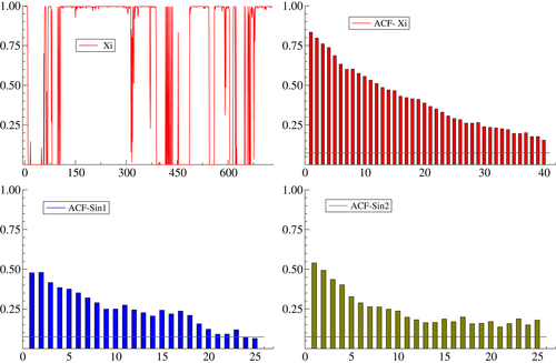
Although the static mixture model can be ruled out from the correlogram of the raw data, it is nevertheless informative about the regimes. Numerically optimizing the log-likelihood function gave the values in the first row of Table II, that is ${\tilde{μ}}_{1} = 4.051$ $(0.014), {\tilde{μ}}_{2} = 1.055$ $(0.056), {\tilde{υ}}_{1} = 12.68, {\tilde{υ}}_{2} = 2.08$ and $\tilde{ξ} = 0.66;$ note that $υ = \ln$ $ω_{ζ} .$ The log-likelihood, in Table I, is $- 816.8,$ which is far lower than we obtained for the single regime dynamic model reported in Section 2.4, and the $Q$ -statistics are huge.

The plot of $ξ (y_{t})$ in Figure 2 shows how the contrast between the distributions in the two regimes gives a clear indication of which regime is operative at any one time. The regimes are obviously not determined randomly and the ACF of the $ξ_{i} {(y_{t})}^{'} s$ indicates that a fairly persistent first-order filter, as in (11), is likely to give a good fit. The circular ACFs (CACFs) for the individual regimes in the lower panels indicate persistent dynamics in the location. The correlations between the three scores are not far from zero.

4.2 Dynamic Mixtures

Although the tests indicate dynamics within each regime, it is useful to begin by fitting a pure DAMM, that is one without intra-regime dynamics but with a dynamic equation for $γ_{t | t - 1}$ as in (11). The estimates of $ω_{μ 1},$ $ω_{μ 2},$ $ω_{ζ 1}$ and $ω_{ζ 1}$ are similar to the estimates found for the static mixture model except that the estimate of $ξ$ is, at 0.90, somewhat higher than the static estimate of 0.66. The log-likelihood is $- 483.1$ so there is a clear improvement over the static mixture model.

The diagnostic test based on the switching residuals, shown in the column headed $γ$ in Table III, indicates that most of the dynamic movements have been captured by the regime-switching equation. However, the $Q$ -statistics for location dynamics remain very high in both regimes; indeed the correlograms are not dissimilar to those in Figure 2. Both are consistent with a first-order dynamic model, (14), for each regime.

Fitting an HMM gives a result very close to that of the DAMM. The log-likelihood is slightly lower, at $- 490.5$ , but the AIC and BIC are slightly bit smaller, reflecting the fact that the HMM has one fewer parameter. The finding that the pure switching model is inadequate is important because most, if not all, of the research in this area has been restricted to pure Markov switching models. Indeed only three pages are devoted to intra-regime dynamics in the book by Zucchini et al. (2016, pp. 150–2).

4.3 Dynamic Mixture Model with Intra-regime Dynamics

The first-order score-driven models for the location in each regime are as in (14) with

u_{i, t} = ξ_{i, t | t} υ_{i, t | t - 1} \sin (y_{t} - μ_{i, t | t - 1}), i = 1, 2,

where

υ_{i, t | t - 1}

is the filtered concentration when the model takes account of heteroscedasticity. The results, for the models labelled (3) and (4), show the dynamics to be fairly persistent in both regimes, with

ϕ_{1}

and

ϕ_{2}

of (14) always above 0.9. The mean of location in the second regime has increased to 3.165 but if it is constrained to its value for the static model, that is 1.05, the log-likelihood is much lower at

- 279.3

as opposed to

- 234.3

for the unconstrained model. It seems that the parameters in the second regime are more difficult to estimate than those in the first, perhaps because the concentration is lower. Nevertheless there is a huge increase in the likelihood as compared with the pure DAMM.

The diagnostics show that serial correlation in location has been eliminated. However, the scores for concentration indicate dynamics. When, in the last line, the model is extended to allow for heteroscedasticity, there is a further improvement in goodness of fit and the level in regime 2 falls to 2.31. On the other hand the underlying probability of being in regime 1, that is $ξ,$ rises from 0.767 to 0.849.

Finally the likelihoods for the two switching models with intra-regime dynamics are, as expected, much bigger than those of the corresponding single regime models and, despite the extra parameters, the AICs and BICs are much smaller.

5 MODELING THE CYLINDER

A bivariate distribution for a circular and a linear variable takes the form of a cylinder. This section shows how a dynamic model can be constructed. The last subsection makes the extension to a bivariate regime switching model.

5.1 Weibull–von Mises (Abe-Ley) Distribution

The Weibull–Sine Skewed–von Mises (WeiSSVM) proposed3by Abe and Ley (2017) combines a von Mises circular distribution for a circular variable,

y,

with a Weibull distribution for a non-negative linear variable,

x

. The skewing term will be dropped here to simplify the exposition, giving the Weibull–von Mises (WeiVM) distribution

\begin{align} f (y, x) & = \frac{α \exp (- α λ)}{2 π \cosh υ} x^{α - 1} \exp {- {(x / \exp λ)}^{α} (1 - \tanh υ . \cos (y - μ))}, \\ - π & \leq y, μ < π, x \geq 0, α > 0, υ \geq 0, \end{align}

where

\exp (λ)

is the scale,

φ

, for the linear variable and

υ

is a parameter that determines concentration for

y

5.2 Dynamic Model

In the dynamic score-driven cylinder model the parameters

μ

and

λ

change over time and the logarithm of the joint density of the conditional WeiVM distribution is

\begin{align} \ln f (y_{t}, x_{t}; μ_{t | t - 1}, λ_{t | t - 1}, ψ) & = \ln (α / 2 π) - \ln \cosh υ - α λ_{t | t - 1} + (α - 1) \ln x_{t} \\ - {(x_{t} / \exp λ_{t | t - 1})}^{α} (1 - \tanh υ \cos (y_{t} - μ_{t | t - 1})), t = 1, \dots, T, \end{align}

(18)

with

- π \leq y_{t} < π,

but with no corresponding restriction on

μ_{t | t - 1};

ψ

denotes the parameters

υ

and

α

and those in the dynamic equations. The conditional scores are

\frac{\partial \ln f_{t | t - 1}}{\partial μ_{t | t - 1}} = u_{t}^{μ} = \tanh (υ) {(x_{t} / \exp λ_{t | t - 1})}^{α} \sin (y_{t} - μ_{t | t - 1})

(19)

and

\frac{\partial \ln f_{t | t - 1}}{\partial λ_{t | t - 1}} = u_{t}^{λ} = α {(x_{t} / \exp λ_{t | t - 1})}^{α} (1 - \tanh (υ) \cos (y_{t} - μ_{t | t - 1})) - α .

(20)

The filters for

μ_{t | t - 1}

and

λ_{t | t - 1}

are driven by

u_{t}^{μ}

and

u_{t}^{λ}

and so for first-order dynamics

\begin{align} μ_{t + 1 | t} & = (1 - ϕ_{μ}) ω_{μ} + ϕ_{μ} μ_{t | t - 1} + κ_{μ} u_{t}^{μ}, \\ λ_{t + 1 | t} & = (1 - ϕ_{λ}) ω_{λ} + ϕ_{λ} λ_{t | t - 1} + κ_{λ} u_{t}^{λ} . \end{align}

(21)

with

μ_{1 | 0} = ω_{μ}

and

λ_{1 | 0} = ω_{λ} .

Both $u_{t}^{μ}$ and $u_{t}^{λ}$ retain the univariate circularity property of being unchanged when multiples of $2 π$ are added or subtracted from $y_{t} .$ The circularity of the scores confirms that when a dynamic score-driven model for a WeiVM distribution, $f (z_{t}, x_{t})$ , allows $z_{t}$ to range over the whole real line, it may be wrapped, as in (2), to give a likelihood function, based on (18), that is the same as that of the (infeasible) likelihood function for $f (z_{t}, x_{t})$ .

Basing the dynamics for

μ_{t | t - 1}

and

λ_{t | t - 1}

on scores means that their movements interact with each other in a way that makes sense given the structure of the WeiVM bivariate distribution. It follows from Abe and Ley (2017) that the distribution of

y_{t}

conditional on

x_{t},

together with all the information at time

t - 1,

v M

with mean

μ_{t | t - 1}

and concentration

υ (x_{t}) = (\tanh υ) . {(x_{t} / \exp λ_{t | t - 1})}^{α},

(22)

so the more

x_{t}

exceeds its expected value, the higher the concentration. Thus (19) can be written as

u_{t}^{μ} = υ (x_{t}) \sin (y_{t} - μ_{t | t - 1})

. When

x_{t}

is close to zero, there is no clear direction so the concentration is low. The conditional distribution of

x_{t}

given

y_{t}

together with all the information at time

t - 1

is Weibull with scale

φ (y_{t}) = {(1 - \tanh υ . \cos (y_{t} - μ_{t | t - 1}))}^{- 1 / α} φ_{t | t - 1},

(23)

where

φ_{t | t - 1} = \exp (λ_{t | t - 1})

. Substituting in (20) gives

u_{t}^{λ} = α [{(x_{t} / φ (y_{t}))}^{α} - 1]

. When

y_{t}

is close to

μ_{t | t - 1}

it will boost the effect of

x_{t} .

5.3 Heteroscedasticity

As the model stands, concentration,

υ (x_{t})

, changes only with

x_{t},

depending on whether

x_{t}

is higher or lower than expected given

λ_{t | t - 1}

. Using a result in Abe and Ley (2017, p. 95), the expected value of

υ (x_{t})

based on information at time

t - 1

\begin{align} E_{t - 1} υ (x_{t}) & = \tanh (υ) E_{x} {(x_{t} / \exp λ_{t | t - 1})}^{α} = \tanh υ \cosh υ . P_{1}^{0} (\cosh υ) \\ = \tanh υ \cosh^{2} υ = 0.5 \sinh (2 υ), \end{align}

where

P_{ν}^{0} (.)

is the associated Legendre function of the first kind with degree

ν

and order zero. Thus the prediction of

υ (x_{t})

is constant. It is not dependent on

λ_{t | t - 1}

and so if, in the context of wind, speed has been high for some time, a value of

x_{t}

lower than its expectation will imply that concentration is suddenly lower than average. This seems implausible and it points to the need to introduce dynamic heteroscedasticity into the model by letting

υ

be dynamic. The score with respect to this new dynamic parameter, denoted,

υ_{t | t - 1},

u_{t}^{υ} = {(x_{t} / \exp λ_{t | t - 1})}^{α} [1 - \tanh^{2} υ_{t | t - 1}] \cos (y_{t} - μ_{t | t - 1}) - \tanh υ_{t | t - 1} .

(24)

The score

u_{t}^{υ}

is very close to that of

λ_{t | t - 1},

in (20), but it differs in that when

y_{t}

is close to

μ_{t | t - 1}

it increases whereas

u_{t}^{λ}

reacts in the opposite direction. Note that

u_{t}^{λ}

is now defined with

\tanh υ_{t | t - 1}

replacing

\tanh υ .

Using the filter for

υ_{t | t - 1}

now gives

E_{t - 1} υ (x_{t}) = 0.5 \sinh (2 υ_{t | t - 1}) .

The heteroscedastic dynamic model includes an equation for $ζ_{t | t - 1} = \ln υ_{t | t - 1}$ to complement those in (21). The information matrix for $μ, λ$ and $ζ$ is given in the Supporting information. Its availability raises the possibility of pre-multiplying the scores by its inverse, as is often done in the dynamic score literature.

Remark 2.Abe and Ley (2017, pp. 96–7), p 96-7, give a generalization,4 the GGSSVM, in which the generalized gamma (GG) distribution replaces the Weibull; the circular marginal distribution is then the Jones-Pewsey distribution. Imoto et al. (2019) propose a generalized Pareto-type cylindrical distribution that can handle heavier tails. In both cases a score driven model can again be formulated.

5.4 Forecasts

Forecasts are based on information at

T

so for

T + 1

we plug

μ_{T + 1 | T}, υ_{T + 1 | T}

and

λ_{T + 1 | T}

into the joint distribution. The (marginal) distribution of

y_{T + 1}

, conditional on information at time

T,

is wrapped Cauchy that is

f_{T} (y_{T + 1}) = \frac{1}{2 π} \frac{1 - \tanh^{2} (υ_{T + 1 | T} / 2)}{1 + \tanh^{2} (υ_{T + 1 | T} / 2) - 2 \tanh (υ_{T + 1 | T} / 2) \cos (y_{T + 1} - μ_{T + 1 | T})},

(25)

where

- π \leq y_{T + 1} < π

. The one-step ahead forecast for direction,

E_{T} (y_{T + 1})

, is just the predicted location

μ_{T + 1 | T}

. The marginal distribution for the linear variable is given in Abe and Ley (2017, p. 94) as

f_{T} (x_{T + 1}) = V_{T + 1 | T} (x_{T + 1}) \frac{α}{e^{λ_{T + 1 | T}}} {(\frac{x_{T + 1}}{e^{λ_{T + 1 | T}}})}^{α - 1} \exp (- {(x_{T + 1} / e^{λ_{T + 1 | T}})}^{α}),

where

0 \leq x_{T + 1} < \infty

and

V_{T + 1 | T} (x_{T + 1}) = \frac{I_{0} ({(x_{T + 1} / e^{λ_{T + 1 | T}})}^{α} \tanh υ_{T + 1 | T})}{\cosh υ_{T + 1 | T}} .

The one-step ahead forecast of

x_{T + 1}

E_{T} (x_{T + 1}) = \exp (λ_{T + 1 | T}) Γ (1 + 1 / α) [{(\cosh υ_{T + 1 | T})}^{1 / α} P_{1 / α} (\cosh υ_{T + 1 | T})] .

Except for the normalizing term

V_{T + 1 | T} (x_{T + 1})

, the form of

f_{T} (x_{T + 1})

is that of a Weibull distribution and likewise

E_{T} (x_{T + 1})

is as for a Weibull distribution, apart from the term in square brackets. Multi-step forecasts can be obtained by simulation. Abe and Ley (2017, p. 94), provide details on how to simulate from the WeiSSVM distribution.

5.5 Switching Cylinders

DAMMs can be applied to multivariate series as in Catania (2021, eq. (3)). In a bivariate model the switching filter for

ξ_{t | t - 1}

depends on the joint PDF

f (y_{t}, x_{t})

. All parameters, including those that are fixed, such as

α,

are regime dependent. Following on from (17 ), the score for location within a regime is then given by

u_{i t}^{μ} = \frac{\partial \ln f_{t | t - 1}}{\partial μ_{i, t | t - 1}} = ξ_{i, t | t} (y_{t}, x_{t}) υ_{i} (x_{t}) \sin (y_{t} - μ_{i, t | t - 1}), i = 1, 2,

where

υ_{i} (x_{t}) = \tanh (υ_{i}) {(x_{t} / \exp λ_{i, t | t - 1})}^{α_{i}},

and similarly for the other scores.

The graphs in Figure 1 suggest that the regimes for direction are more clearly defined than those for speed. Thus it is worth considering whether to model regime switching only in terms of the marginal distribution of direction, $y_{t}$ . To implement such a regime switching mechanism, the PDF in the score with respect to the dynamic switching probability, that is (11), is taken to be wrapped Cauchy, as in (25), and the same density is used in the contemporaneous probability (13).

6 WIND DIRECTION AND SPEED IN GALICIA

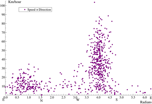
The scatter plot of speed and direction for the Galicia data in Figure 3 highlights the regimes in direction and confirms the impression gained from Figure 1 that speed tends to be higher when the wind is coming from the SW.

As might be expected from the univariate results on wind direction, a static mixture model fares badly, with $\ln L = - 3732.2$ as opposed to $\ln L = - 3371.2$ for the single regime model without heteroscedasticity and $\ln L = - 3355.7$ with heteroscedasticity. The pure DAMM model, shown in the second line of Table IV and labelled model (6), is much better, with $\ln L = - 3413.7$ but it too fails to beat the single regime models. The score-based $Q$ -statistics for residual serial correlation shown in Table VI are huge.

Table IV. Goodness of fit of the two regime WeiVM model with the estimated dynamic parameters of the switching probability from fitting, (5), the static mixture model, (6), the pure DAMM model, (7), the DAMM model with intra regime dynamic location and scale and (8), DAMM model with intra regime dynamic location, scale and concentration

Model	AIC	BIC	Logl	$ω_{γ}$	$ϕ_{γ}$	$κ_{γ}$	$ξ$
(5)	7,482.446	7,523.954	$- 3, 732.223$	0.994	–	–	0.730
(5)	7,482.446	7,523.954	$- 3, 732.223$	(0.097)			0.730
(6)	6,849.460	6,900.193	$- 3, 413.730$	1.084	0.846	11.079	0.747
(6)	6,849.460	6,900.193	$- 3, 413.730$	(0.552)	(0.022)	(1.224)	0.747
(7)	6,034.761	6,122.389	$- 2, 998.380$	1.151	0.924	7.729	0.760
(7)	6,034.761	6,122.389	$- 2, 998.380$	(0.664)	(0.015)	(1.114)	0.760
(8)	5,992.685	6,098.762	$- 2, 973.343$	1.669	0.870	27.487	0.842
(8)	5,992.685	6,098.762	$- 2, 973.343$	(0.561)	(0.020)	(0.833)	0.842
(9)	6,018.408	6,106.037	$- 2, 990.204$	1.336	0.966	5.594	0.792
(9)	6,018.408	6,106.037	$- 2, 990.204$	(0.828)	(0.010)	(1.076)	0.792
(10)	5,939.650	6,045.727	$- 2, 946.825$	0.032	0.879	15.945	0.508
(10)	5,939.650	6,045.727	$- 2, 946.825$	(0.552)	(0.016)	(2.524)	0.508

Note: Models (9) and (10) are specified in the same way as (7) and (8) except that the switching probability is driven by the marginal distribution with respect to location. The switching parameters are shown in the last four columns, with $ξ$ denoting the logistic transformation of $ω_{γ}$ .

The inclusion of dynamics within regimes offers considerable improvement. As before the fit is better with heteroscedasticity dynamics. The main issue to resolve is whether the dynamics in the switching equation should depend on both direction and speed or on direction only. The results favour the second possibility, especially when the dynamics include heteroscedasticity. Thus the estimates reported in the last lines of Tables IV–VI are for the preferred model. As can be seen, $\ln L = - 2946.8$ . There is still some residual serial correlation in some of the components, but, as noted earlier, this is not unusual with large sample sizes. The estimates of $α$ in the Weibull parameter are well above one in almost all cases.

Table V. Estimated dynamic parameters for the two regime WeiVM model from fitting, (5), the static mixture model, (6), the pure DAMM model, (7), the DAMM model with intra regime dynamic location and scale and (8), DAMM model with intra regime dynamic location, scale and concentration

Model	$ω_{μ 1}$	$ϕ_{μ 1}$	$κ_{μ 1}$	$ω_{λ 1}$	$ϕ_{λ 1}$	$κ_{λ 1}$	$ω_{γ 1}$	$ϕ_{γ 1}$	$κ_{γ 1}$	$α_{1}$	$ω_{μ 2}$	$ϕ_{μ 2}$	$κ_{μ 2}$	$ω_{λ 2}$	$ϕ_{λ 2}$	$κ_{λ 2}$	$ω_{γ 2}$	$ϕ_{γ 2}$	$κ_{γ 2}$	$α_{2}$
(5)	4.046	–	–	2.418	–	–	0.695	–	–	2.115	0.886	–	–	1.561	–	–	0.543	–	–	2.021
(5)	(0.012)			(0.054)			(0.024)			(0.033)	(0.028)			(0.096)			(0.051)			(0.057)
(6)	4.048	–	–	2.422	–	–	0.735	–	–	2.171	0.917	–	–	1.732	–	–	0.381	–	–	2.002
(6)	(0.011)			(0.045)			(0.022)			(0.029)	(0.032)			(0.025)			(0.047)			(0.041)
(7)	4.002	0.927	0.010	2.218	0.978	0.021	0.748	–	–	3.575	1.694	0.992	0.043	1.622	0.811	0.089	0.489	–	–	2.329
(7)	(0.032)	(0.025)	(0.002)	(0.080)	(0.005)	(0.002)	(0.021)			(0.029)	(0.110)	(0.003)	(0.007)	(0.016)	(0.047)	(0.010)	(0.041)			(0.031)
(8)	4.048	0.941	0.008	2.161	0.976	0.023	0.592	0.912	0.015	3.398	0.854	0.982	0.013	1.798	0.802	0.046	1.261	0.998	0.067	2.342
(8)	(0.001)	(0.024)	(0.001)	(0.124)	(0.000)	(0.002)	(0.027)	(0.027)	(0.003)	(0.054)	(0.071)	(0.019)	(0.004)	(0.002)	(0.068)	(0.006)	(0.133)	(0.000)	(0.014)	(0.033)
(9)	3.998	0.919	0.010	2.274	0.972	0.027	0.744	–	–	3.478	1.408	0.967	0.052	1.482	0.924	0.051	0.485	–	–	2.481
(9)	(0.030)	(0.025)	(0.002)	(0.110)	(0.007)	(0.003)	(0.020)			(0.031)	(0.082)	(0.013)	(0.011)	(0.166)	(0.038)	(0.010)	(0.053)			(0.047)
(10)	4.068	0.957	0.007	2.326	0.972	0.018	–0.447	0.941	0.025	3.237	1.786	0.993	0.039	1.401	0.943	0.038	–0.479	0.756	0.021	2.559
(10)	(0.042)	(0.016)	(0.001)	(0.091)	(0.008)	(0.002)	(0.061)	(0.015)	(0.005)	(0.033)	(0.200)	(0.004)	(0.007)	(0.170)	(0.023)	(0.006)	(0.053)	(0.103)	(0.010)	(0.048)

Note: Models (9) and (10) are specified in the same way as (7) and (8) except that the switching probability is driven by the marginal distribution with respect to location.

Table VI. Box–Ljung test with

P = 5, Q (5)

, for residual correlation on the fitted scores from fitting, (5), the static mixture model, (6), the pure DAMM model, (7), the DAMM model with intra regime dynamic location and scale and (8), DAMM model with intra regime dynamic location, scale and concentration

Model	$μ_{1}$	$λ_{1}$	$ζ_{1}$	$μ_{2}$	$λ_{2}$	$ζ_{2}$	$γ$
(5)	$767.82 6^{* * *}$	$774.36 6^{* * *}$	$2037.3 6^{* * *}$	$550.02 1^{* * *}$	$649.58 6^{* * *}$	$1248.8 6^{* * *}$	$2642.1 3^{* * *}$
(6)	$753.42 5^{* * *}$	$678.76 6^{* * *}$	$1918.0 3^{* * *}$	$587.87 0^{* * *}$	$516.35 5^{* * *}$	$1339.6 6^{* * *}$	$26.82 7^{* * *}$
(7)	5.093	3.303	$219.27 0^{* * *}$	$25.64 6^{* * *}$	$14.79 2^{* *}$	$159.49 4^{* * *}$	$11.66 6^{* *}$
(8)	3.479	3.737	$38.26 5^{* * *}$	$53.01 2^{* * *}$	6.806	$41.57 9^{* * *}$	1.069
(9)	3.459	1.528	$158.64 4^{* * *}$	$25.68 6^{* * *}$	$10.49 6^{*}$	$141.56 6^{* * *}$	$120.99 5^{* * *}$
(10)	$10.29 8^{*}$	2.551	$26.70 6^{* * *}$	$26.68 4^{* * *}$	5.073	$54.87 5^{* * *}$	$43.29 4^{* * *}$

Note: Models (9) and (10) are specified in the same way as (7) and (8) except that the switching probability is driven by the marginal distribution with respect to location. (Nominal) significance levels: 0.01 ‘***’, 0.05 ‘**’, 0.1 ‘*’.

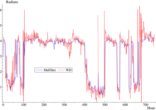
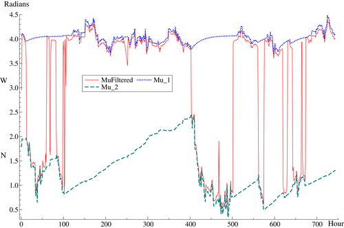
The observations and combined filters for direction are shown in Figure 4. The filtered estimates are smoother than the raw observations. The filtered estimates stay well within the range $[0, 2 π)$ whereas the observations sometimes move rapidly between the top and bottom of the graph. 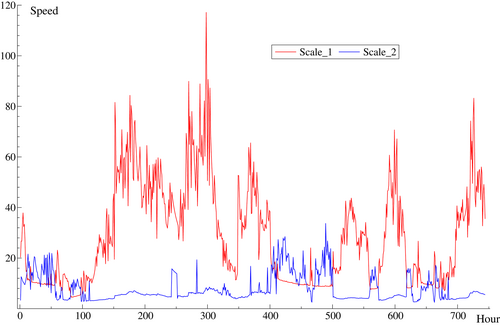Note that the combined filter for mean direction is computed using the $a \tan 2$ function, as in (17), while the corresponding filter for scale is $ξ_{1, t | t - 1} \exp (λ_{1, t | t - 1}) + ξ_{2, t | t - 1} \exp (λ_{2, t | t - 1}), t = 1, \dots, T .$

Figures 5 and 6 show filtered wind direction and speed in individual regimes. It can be seen that when the probability of being in a given regime is small, the movements in the underlying filter change only gradually. For wind direction, the combined filter of Figure 4 is also shown. The combined filter for speed is not shown as it is just the sum of the individual filters.

Remark 3.When there is no wind, it has no direction. In such cases $x_{t} = 0$ and so the model gives $υ (x_{t}) = 0$ which implies the (unobserved) wind direction is distributed uniformly. It is evident from (20) that the score for location, $u_{t}^{μ},$ is zero. Thus the observation is effectively ignored as in the naive solution for dealing with an observation that is missing.5 This is not the case for the scale of the linear variable because $u_{t}^{λ} = - α$ and the concentration score where $u_{t}^{υ} = - \tanh υ_{t | t - 1} .$ As regards the likelihood, the difficulty is that $f (y_{t}, 0) = 0$ for $α > 1,$ indicating that $x_{t} = 0$ is impossible. For $α < 1,$ $f (0) = \infty$ which is also unhelpful. Only for $α = 1$ is there a viable solution as in this case $f (y_{t}, 0) = 1 / 2 π .$ The simplest solution is to assume there is no contribution to the likelihood.

7 CONCLUSION

Score-driven regime switching models can be extended to handle circular observations and diagnostic tests can be constructed. The models allow for changing concentration as well as changing location. When fitted to hourly wind direction in a site in Galicia, pure regime switching models, without intra-regime dynamics, are unable to outperform the single regime model when both location and scale are dynamic. Although the diagnostic test based on the switching residuals indicates that there are no omitted dynamics in the regime-switching equation, the $Q$ -statistics for location dynamics are still highly significant in both regimes. Fitting a score-driven switching model with location dynamics in each regime gives a big increase in the likelihood function.

The score-driven approach is then used to construct dynamic bivariate models for circular and linear variables with a conditional cylindrical distribution. The preferred specification for the Galicia data has dynamic location and concentration for wind direction and dynamic location/scale for its speed. Estimating a restricted regime switching model, in which the regime dynamics depend only on direction, gives a good fit when heteroscedasticity is included and the resulting filter for direction tracks the observations remarkably well. Again the modelling of intra-regime dynamics is crucial.

There is further scope for research extending the score-driven approach to bivariate dynamic cylindrical models based on copulas, as used by García-Portugués et al. (2013) and Lagona (2019), and to directional data on a sphere or torus.

ACKNOWLEDGEMENTS

We are grateful to Eduardo García-Portugués for providing the Galicia data used in García-Portugués et al. (2013). Earlier versions of some of the ideas in this article were presented at the Econometric Models of Climate Change conference in Milan in August 2019, at the 22nd Oxmetrics conference at Nuffield college, Oxford in September, 2019, and at workshops in Cambridge, Bologna, Ecole Polytechnique Féd érale de Lausanne, the QUT Centre for Data Sciences and the University of Konstanz. Later versions were given at a plenary (virtual) session of the 45th NBER-NSF conference in October 2021 at Rice University, Houston and at the ADISTA22 (Advances in Directional Statistics) conference in Santiago de Compostela in June 2022. We are grateful to Anthony Davison, Jurgen Doornik, David Hendry, Stan Hurn, Peter Jupp, John Kent, Francisco Lagona, Rutger-Jan Lange, Christophe Ley, Ken Lindsay, Oliver Linton, Alessandra Luati, Paul Myer, Alexiy Onatski, Richard Smith, Howell Tong and two referees for helpful comments.

Open Research

DATA AVAILABILITY STATEMENT

The data that support the findings of this study are available from the corresponding author on reasonable request.

Supporting Information

References

Abe T, Ley C. 2017. A tractable, parsimonious and flexible model for cylindrical data, with applications. Econometrics and Statistics 4: 91–104.
10.1016/j.ecosta.2016.04.001
Web of Science® Google Scholar
Breckling J. 1989. The analysis of directional time series: Applications to wind speed and direction.
Google Scholar
Calvori F, Creal D, Koopman S, Lucas A. 2017. Testing for parameter instability in competing modeling frameworks. Journal of Financial Econometrics 15: 223–246.
Web of Science® Google Scholar
Catania L. 2021. Dynamic adaptive mixture models with an application to volatility and risk. Journal of Financial Econometrics 19: 531–564.
10.1093/jjfinec/nbz018
Web of Science® Google Scholar
Creal D, Koopman S, Lucas A. 2013. Generalized autoregressive score models with applications. Journal of Applied Econometrics 28: 777–795.
10.1002/jae.1279
Web of Science® Google Scholar
Fisher N, Lee A. 1992. Regression models for an angular response. Biometrics 48: 665–677.
10.2307/2532334
Web of Science® Google Scholar
Fisher N, Lee A. 1994. Time series analysis of circular data. Journal of the Royal Statistical Society B(70): 327–332.
Google Scholar
García-Portugués E, Barros A, Crujeiras R, González-Manteiga W, Pereira JC. 2014. A test for directional-linear independence, with applications to wildfire orientation and size. Stochastic Environmental Research and Risk Assessment 28: 1261–1275.
10.1007/s00477-013-0819-6
Web of Science® Google Scholar
García-Portugués E, Crujeiras R, González-Manteiga W. 2013. Exploring wind direction and so 2 concentration by circular-linear density estimation. Stochastic Environmental Research and Risk Assessment 27: 1055–1067.
10.1007/s00477-012-0642-5
Web of Science® Google Scholar
Haas M, Mittnik S, Paolella M. 2004. A new approach to Markov-switching garch models. Journal of Financial Econometrics 2: 493–530.
10.1093/jjfinec/nbh020
Google Scholar
Hamilton J. 1989. A new approach to the economic analysis of nonstationary time series and the business cycle. Econometrica 57(2): 357–384.
10.2307/1912559
Web of Science® Google Scholar
Hamilton J. 1994. Time series analysis.
Google Scholar
Hamilton J. 1996. Specification testing in Markov-switching time-series models. Journal of Econometrics 70: 127–157.
10.1016/0304-4076(69)41686-9
Web of Science® Google Scholar
Harvey A, Hurn S, Palumbo D, Thiele S. 2022. Modeling circular time series. mimeo. Revised version of a 2019 Cambridge Working Papers in Economics. Mimeo (1971).
Google Scholar
Harvey A, Thiele S. 2016. Testing against changing correlation. Journal of Empirical Finance 38: 575–589.
10.1016/j.jempfin.2015.09.003
Web of Science® Google Scholar
Harvey AC. 2013. Dynamic models for volatility and heavy tails: with applications to financial and economic time series. Econometric Society Monograph.
Google Scholar
Holtzmann H, Munk A, Suster M, Zucchini W. 2006. Hidden Markov models for circular and linear-circular time series. Environmental and Ecological Statistics 13: 325–347.
10.1007/s10651-006-0015-7
Web of Science® Google Scholar
Imoto T, Shimizu K, Abe T. 2019. A cylindrical distribution with heavy-tailed linear part. Japanese Journal of Statistics and Data Science 2: 129–154.
10.1007/s42081-019-00031-5
Google Scholar
Jammalamadaka S , SenGupta A. 2001. Topics in circular statistics.
Google Scholar
Jones M, Pewsey A. 2005. A family of symmetric distributions on the circle. Journal of the American Statistical Association 100: 1422–1428.
10.1198/016214505000000286
CAS Web of Science® Google Scholar
Lagona F. 2019. Copula-based segmentation of cylindrical time series. Statistics and Probability Letters 144: 16–22.
10.1016/j.spl.2018.04.011
Web of Science® Google Scholar
Lagona F, Picone M, Maruotti A. 2015. A hidden Markov model for the analysis of cylindrical time series. Environmetrics 26: 534–544.
10.1002/env.2355
Web of Science® Google Scholar
Mardia KV, Jupp P. 2000. Directional statistics.
Google Scholar
Pewsey A, García-Portugués E. 2021. Recent advances in directional statistics. TEST 30: 1–58.
10.1007/s11749-021-00759-x
Web of Science® Google Scholar
Smith D. 2008. Evaluating specification tests for Markov-switching time-series models. Journal of Time Series Analysis 29: 629–652.
10.1111/j.1467-9892.2008.00575.x
Web of Science® Google Scholar
Waltz R, Morales J, Nocedal J, Orban D. 2006. An interior algorithm for nonlinear optimization that combines line search and trust region steps. Mathematical Programming 107: 391–408.
10.1007/s10107-004-0560-5
Web of Science® Google Scholar
Zucchini W, MacDonald IL, Langrock R. 2016. Hidden Markov models for time series: an introduction using r. Monographs on Statistics and Applied Probability 150.
Google Scholar

1 Score-driven time series models were developed by Harvey (2013) and Creal et al. (2013), where they were called DCS and GAS models respectively.
2 The fact that the range of the observations is $[0, 2 π)$ rather than $[- π, π)$ makes no substantive difference to the results.
3 Abe and Ley (2017) have $β = \exp (- λ)$ and $κ = υ .$
4 Note that they have $α$ replacing our $α γ$ and $γ$ replacing $α .$
5 There is a run of missing observations on both wind and velocity around observation 250. In such cases we set all scores to zero: hence the slight dip in Figures 5 and 6. There are a few more missing observations around 455 and 680.

Volume44, Issue4

July 2023

Pages 374-392

Regime switching models for circular and linear time series

Abstract

1 INTRODUCTION

2 SCORE-DRIVEN MODELS FOR CIRCULAR DATA

2.1 Dynamic Location

2.2 Tests

2.3 Heteroscedasticity

2.4 Application to Circular Data from Galicia

3 SWITCHING REGIMES

3.1 Static Mixture Model

3.2 Dynamic Mixture Model

3.3 Dynamics Within Regimes

3.4 Model Selection and Diagnostics

3.5 Circular Mixture Models

4 SWITCHING MODELS FOR GALICIA

4.1 Static Mixture

4.2 Dynamic Mixtures

4.3 Dynamic Mixture Model with Intra-regime Dynamics

5 MODELING THE CYLINDER

5.1 Weibull–von Mises (Abe-Ley) Distribution

5.2 Dynamic Model

5.3 Heteroscedasticity

5.4 Forecasts

5.5 Switching Cylinders

6 WIND DIRECTION AND SPEED IN GALICIA

7 CONCLUSION

ACKNOWLEDGEMENTS

Open Research

DATA AVAILABILITY STATEMENT

Supporting Information

References

Figures

References

Information

About Wiley Online Library

Help & Support

Opportunities

Connect with Wiley

Regime switching models for circular and linear time series

Abstract

1 INTRODUCTION

2 SCORE-DRIVEN MODELS FOR CIRCULAR DATA

2.1 Dynamic Location

2.2 Tests

2.3 Heteroscedasticity

2.4 Application to Circular Data from Galicia

3 SWITCHING REGIMES

3.1 Static Mixture Model

3.2 Dynamic Mixture Model

3.3 Dynamics Within Regimes

3.4 Model Selection and Diagnostics

3.5 Circular Mixture Models

4 SWITCHING MODELS FOR GALICIA

4.1 Static Mixture

4.2 Dynamic Mixtures

4.3 Dynamic Mixture Model with Intra-regime Dynamics

5 MODELING THE CYLINDER

5.1 Weibull–von Mises (Abe-Ley) Distribution

5.2 Dynamic Model

5.3 Heteroscedasticity

5.4 Forecasts

5.5 Switching Cylinders

6 WIND DIRECTION AND SPEED IN GALICIA

7 CONCLUSION

ACKNOWLEDGEMENTS

Open Research

DATA AVAILABILITY STATEMENT

Supporting Information

References

Figures

References

Related

Information