[Correction added on 6 December 2022, after first online publication: The affiliation of the third author, Alan O'Connor, was incorrect in the originally published version of this article. It should be affiliation 3, not 2 and 3. This updated version corrects the mistake.]

Funding information: Interreg, Grant/Award Number: EAPA 45/2018-AAFLOODS

About

Sections

PDF

Tools

Share a link

Email
Wechat
Bluesky

Abstract

Floods represent one of the major challenges facing human societies. The impacts caused by them are extensive, and efficient flood adaptation will play a key role in the current century. The present work proposes a new approach to decision-making in flood adaptation aimed at achieving robust adaptation decisions. It consists in evaluating decisions on a triaxial basis that considers expectation, probability quantile and investment in a so-called expectation–quantile–investment (EQI) evaluation. With such approach it is possible to understand the influence of uncertainties in the probabilistic response of adaptation. While adaptation should minimise expected total costs, it needs also to be robust for competitive levels of investment. Transfer curves that relate events with outcomes are used to infer on the probabilistic character of decisions in a case study of a vulnerable location. Results show that EQI-informed decisions can distinguish optimality in apparently competitive measures. It is shown that decisions based on one-dimensional or two-dimensional aspects of this triaxial rationale may fail to identify important probabilistic outcomes of adaptation, such as, the possibility of large losses with relevant probability of occurrence; and that are of high relevance when uncertainty considerations need to be enclosed in the analysis of adaptation.

1 INTRODUCTION

Floods represent one of the major challenges facing future human societies. Floods are the most prevalent natural disaster (Jha et al., 2012), and the current expectation is for their frequency and intensity to increase in the future (Arias et al., 2021) due to climate change (Vanneuville et al., 2016). The expectation of losses due to flooding is significant. In Europe, failure to mitigate river flood risk alone can result in increases of losses by a factor of up to six in the present century, with current estimates for loss at 7.8b€ if no further changes in climate occur (Dottori et al., 2020). Trends in flood zone urbanisation have been similarly steep and continue to climb worldwide (Jongman et al., 2012). More human assets are getting in the way of future floods and could potentially create additional flooding issues due to an increase of non-permeable surfaces and lack of natural drainage as a result of urbanisation activities (Jongman, 2018). As a result, adaptation to flooding has become one of the most urgent issues for current societies, and examples of such are the commitment to it illustrated by overarching initiatives such as the EU Floods Directive (European Commission, 2007) or the directive's lead flooding management initiatives.

Mapping flood risks is a common approach used to mitigate and manage floods. It raises awareness about the exposure and vulnerability of flood-prone areas and informs decisions. In practice, flooding events and exceedance of water depths are combined with some form of vulnerability assessment to define levels of risk that are mapped for different regions. This involves estimating the probability of a certain water discharge, using it to estimate water levels, then translating these into a form of damage, and finally assessing its probability or the probability of the associated risk (Salman and Li, 2018).

A significant portion of recent research in this context has been directed at addressing how assessment can be defined through investigation of topics such as, new modelling techniques, application to sites or assessment of consequences (Morrison et al., 2018; Rehman et al., 2019). While such tools are key to support decision processes, only limited research has been directed at the decision frameworks and the different considerations that affect these. Uncertainty in particular has large influence on decision-making and its outcomes. It has origin on multiple factors, and can be separated in two major dimensions, aleatory and epistemic. Examples of aspects that contribute to uncertainty in flood assessment and management are, lack of long-enough and reliable observational records, improper assumption of flood frequency distributions, uncertainty in land use, damage models and inundation depth on flood damage estimates or selection of appropriate methods for estimation of extremes (Salman and Li, 2018).

The present work discusses a new approach to address decision making under uncertainty in flood adaptation using a probabilistically informed decision scheme. A representative study is used to discuss optimal decision-making in adaptation that combines probabilistic criteria and investment in an expectation–quantile–investment (EQI) evaluation. The idea of an EQI analysis is that decisions to flood adaptation should be performed at least on a tridimensional space where expectations of net-costs are evaluated alongside with their probabilistic deviations and combined with an analysis of investment.

For such, Section 2 focuses on decision-making based on probabilistic considerations; Section 3 discusses the main optimal decision framework that enables a probabilistic analysis and a triaxial approach to decision; Section 4 examines and discusses the proposed approach applied in an illustrative case study; and, finally, the main conclusions of the work developed are presented in Section 5.

2 ADAPTATION TO FLOODING USING A PROBABILISTIC ANALYSIS

Adaptation to flooding has been a major topic of research in recent years, and addressing uncertainty has become a key challenge in this regard. In an uncertainty assessment of flooding adaptation, a scenario-based approach or sensitivity analysis can be applied. Alternatively, a probabilistic analysis may be used, where different uncertainties are characterised to study probable outcomes for specified decisions. This involves defining a joint probability of input variables that then propagates through the assessment to the outcomes. The type of uncertainty being addressed will also play a major role, whether it can be characterised or not, in the outcomes. Hall and Solomatine (2008) provide a comprehensive analysis of how uncertainty in flooding adaptation is assessed, proposing a sequential framework to address it. The authors make insightful remarks in this regard, such as the importance of a probabilistic representation of outcomes and the relevance of separating sources of uncertainty and representing these explicitly in this probabilistic evaluation. Jung and Merwade (2012) apply a framework to research the effects of uncertain variables in flooding outcomes showing that inundation areas could vary by 29% in one of the sites studied. Such assessment informs then decisions, most frequently applied as an expectation measure, with common measures used to quantify adaptation being the expected annual benefits or damages (Lasage et al., 2014; Wagenaar et al., 2019; Lorie et al. 2020).

According to Kull et al. (2013), probability distributions are one of the most useful tools to have some probabilistic understanding of flooding adaptation outcomes. They provide estimates of expectation and also carry information on the variability of outcomes for their reference time-period. In Kheradmand et al. (2018) a probabilistic approach is defined that relies on these for a regional study, defining a spectrum of adaptation measures and using an expectation of annual loss as a comparative measure. In Muis et al. (2015) a global approach is used to approximate local adaptation, and large variations are identified in the reduction of expected annual damage for different probabilistic outcomes. In Dittrich et al. (2019), three climate change scenarios are considered as a means of addressing the uncertainty related to the estimation of benefits from flood adaptation. It is noted that while expectation of occurrences provides the most meaningful indicator for decision-making, it has limited information about potential deviations from this reference value. Hall and Solomatine (2008) discuss the importance of analysing the full probability distribution of adaptation for different measures, and highlighting how such analysis can inform robust decisions. Results from the full probabilistic parametric approach of Apel et al. (2006) show that large variability can be found when assessing the probabilistic character of flooding events. Hall and Solomatine (2008) also highlight the need to account for more than expected values in decisions, when introducing the term robust as a decision that functions in a wide range of circumstances.

It is noted that to capture the full probabilistic performance of flood adaptation in decision-making schemes stochastic simulation and programming can provide further insight into probabilistic outcomes. Abadie et al. (2017) apply stochastic simulation in adaptation decision-making, considering uncertainties related to event occurrence and simulating combinations of extreme events as a Poisson process, capturing the variability of events within the considered time-frame. Stochastic programming also allows to capture the variability of an optimal decision with dependence on simulated events, however, its application in the context of flooding has been mainly targeted at relief schemes (Chang et al., 2007; Garrido et al., 2015).

Abadie et al. (2017) in particular apply real options analysis in a context of uncertainty assessment. It was highlighted earlier that the type of uncertainty plays a key role in the assessment of flood adaptation and mitigation, and in this respect, uncertainties can be epistemic or aleatory, and deep or not. Deep uncertainties cannot be characterised in a closed form, that is, have a realistic context but it is not possible to attribute probabilities to them. Handling these has become progressively important in the context of flood adaptation, and present engineering designs are expected to gain from favouring some level of flexibility (De Neufville and Scholtes, 2011), which is supported in the evaluation of Deng et al. (2013), and with different methodologies being defined in the last decade to tackle decision-making that accounts for different types of uncertainty (Helmrich and Chester, 2022). Real options analysis in particular emphasises the optionality of adapting the infrastructure and finding the optimal path of investment, and can handle deep uncertainty as uniformly distributed (Buurman and Babovic 2016). To explicitly handle deep uncertainty, evaluation of dynamic adaptive pathways (Haasnoot et al., 2013) was developed to prioritise flexibility and evaluate the value of decisions considering the expectation of timelines for failure, or so-called ‘tipping points’, and the capability to gain further information valuing the adaptivity to move to an alternative mitigation strategy in the future. Both have been shown to effectively problems with different types of uncertainty and have been driven by flood prevention and mitigation (Manocha and Babovic, 2017).

In the present work, following the discussion of Hall and Solomatine (2008), decision-making for flood adaptation that considers uncertainty through a probabilistic analysis is researched using mathematical programming that considers the probabilistic performance of adaptation. It is the basis for exploring further uncertainties in design (e.g., deep uncertainties) using a triaxial approach with, expectation of risk, quantile of risk and investment. To decrease the effort necessary for a probabilistic analysis such as proposed, transfer curves are discussed to characterise the probabilistic outcomes of adaptation. This rationale follows the work of Kay et al. (2014), where response surfaces are implemented to mitigate the large cost of performing a probabilistic characterisation that compares different scenarios.

3 OPTIMAL PROBABILISTIC ADAPTATION TO FLOODING

A frequent problem setting for adaptation to flooding in a certain location is to have a spectrum of adaptation alternatives that go through a decision-making procedure to investigate their outcomes and the final decision on their implementation. In flood risk management it is common to work with return periods for flooding events and their respective risks (commonly used return periods are the 10, 100 or 500 year flood event) (Salman and Li, 2018) or from a risk-based perspective, with an annual risk expectation (Lendering et al., 2019).

To study different adaptation alternatives there is a need to infer on the effect of adaptation in the flooding event (e.g., if measures that alter the surface flows are used) or risk profiles. This may demand flood modelling within new boundary conditions that may involve performing multiple model evaluations for different return period events.

The motivation to use a transfer function is supported on the fact that only a subset of models or simulations of flooding at different representative return periods may suffice the approximation of outcomes for a certain adaptation measure in a probabilistic analysis. In the context of describing in a probabilistic form events such as maxima this is also valid, and probability distributions that approximate independent maxima in a period of time for order statistics will fall in a family of distributions that are also continuous and can be parameterised (Castillo, 2012).

This rationale can be used to create a series of functions that measure the impact of each alternative in a way that each is associated with event probabilities at a reference time frame. Such curves allow to approximate the outcomes of flooding events by-passing the necessary effort to perform the multiple modelling analyses required in a probabilistic analysis and uncertainty assessment. Therefore, implementation of the EQI evaluation is discussed within the context of using transfer functions.

A transfer function for adaptation can be defined based on the benefit b(a, x) of implementing measure(s) of adaptation a in an event of flooding x. It defines the establishment of a priori mapping of b(a, x) for uncertain or probabilistic conditions of flooding. This mapping enables solving the decision-making as a mathematical programming problem that requires limited effort (it is noted that the amount of effort needed to perform uncertainty characterisation is recurrently highlighted as a limitation in the literature (Kay et al., 2014; Teixeira, O'Connor, & Nogal, 2019)).

z_{a_{i}} \in z_{a}

represents a binary decision variable of implementing an adaptation measure

a_{i} \in a with i \in ℕ^{+}

(or a subset of measures i), from a set of N adaption measures then C(z_a, x) can be defined as

C (z_{a}, x) = \sum_{i = 1}^{N} z_{a_{i}} (Φ (a_{i}, x) + c_{a_{i}}),

(1)

where C(z_a, x) is the net-cost of an adapted outcome with the

z_{a} = [z_{a_{i}}]

decision implemented in a discrete flooding scenario x, and where

c_{a_{i}}

is the metric of value for implementing a_i, and with Φ(a_i, x) being a transfer function for the net-cost of the respective adaptation measure a_i evaluated in x and defined as,

Φ (a_{i}, x) = D (x) - b (a_{i}, x), with a = [a_{i}], i \in ℕ^{+}, \forall x \in ℝ^{+},

(2)

that characterises the outcome of the decision

z_{a_{i}}

if an event x occurs. b(a_i, x) ∈ [0, D(x)] in the current implementation, is the amount of protection, benefit or reduction of D(x) due to the measure(s) a_i, and D(x) is the non-adapted loss at x. An integer linear programming problem to find the optimal adaptation (in terms of net-cost) set of measures based on a flooding event x is also defined as,

\begin{array}{l} \underset{z_{a}}{Minimize} C (z_{a}, x) = \sum_{i = 1}^{N} z_{a_{i}} Φ (a_{i}, x) + \sum_{i = 1}^{N} z_{a_{i}} c_{a_{i}}, \\ with z_{a} = [z_{a_{i}}], a = [a_{i}], i \in ℕ^{+}, \forall x \in ℝ^{+}, \\ Φ (a, x) = [Φ (a_{i}, x)] \in ℝ_{\geq 0}, and \\ c_{a} = [c_{a_{i}}] \in ℝ_{\geq 0} \end{array}

(3)

and can be extended to multiple events to find the z_a that is expected to provide optimal performance to a spectrum of x events,

\begin{array}{l} \underset{z_{a}}{Minimize} \sum_{x} C (z_{a}, x) = \sum_{x} \sum_{i = 1}^{N} z_{a_{i}} Φ (a_{i}, x) + \sum_{i = 1}^{N} z_{a_{i}} c_{a_{i}}, with \\ z_{a} = [z_{a_{i}}], a = [a_{i}], c_{a} = [c_{a_{i}}] \in ℝ_{\geq 0}, i \in ℕ^{+}, \forall x \in ℝ^{+} \end{array}

(4)

where the most protection in adaptation is achieved on a combination of i ≤ n adaptation measures through z_a. Two common constraints in this optimization found in practice are,

\sum_{j} z_{a_{j}} \leq 1, j \subset I = [i] and i \in ℕ^{+},

(5)

which is the case of non-compatible measures, that is, j adaptation measures of the set of all measures I = [i] that cannot be installed simultaneously (e.g., parametric variations of a measure). Or,

\sum_{i} z_{a_{i}} c_{a_{i}} \leq ℬ, ℬ \in ℝ^{+},

(6)

where

ℬ

is the available budget for adaptation. The x characterises discrete flooding events, and each x outcome involves assessing D(x) and then studying the effects of implementing z_a. If different

z_{a_{i}}

have joint effects this can be also accounted for in the binary form vector and transfer function. Such can be done through definition and modelling of adaptation alternatives a_i that account for the combined effects of individual adaptation measures, or using joint or higher dimensional transfer function forms. The x representative of a flooding event is assumed to be always positive and can be considered to take different forms, such as, the annual maxima flooding event that is able to relate Φ through probability. In such circumstance, this formulation reduces to the form of finding the z_a that minimises the expected annual net-cost from flooding, which is discussed in the following section. In the present work metrics of absolute net-cost are considered as being more informative for decision-makers, and in particular when the probabilistic characterisation of adaptation is addressed. This will be further discussed in Section 4.

3.1 Application of probability transfer functions

Following the approach of Section 3 it is then possible to use a combination of flood modelling with probability to research on decision-making that also considers the probabilistic character of the perturbation and (i.e., flooding event) and adaptation. From the uncertainty assessment perspective Φ(a, x) can be also described through the probability of an uncertain event x, p(x). Then,

\begin{array}{l} Φ (a, x) = Φ (a, p (x)), x = F^{- 1} [p (x)], and \\ Φ (a, x) = [Φ (a_{i}, x)] \subset ℝ_{\geq 0}, \end{array}

(7)

with F[x] representing the probability distribution function associated with x, and F⁻¹ its inverse. If F[x] represents the probability distribution function of the annual event x, and X = [x_t] is a realisation of T uncertain x yearly events with associated probability p(X), the mathematical programming problem presented in Equation (4) can be described as a probabilistic adaptation problem using Φ(a, p(x)) for which in any period T an optimal adaptation decision for a realised random X is

\underset{z_{a}}{Minimize} C (z_{a}, p (x), T) = \sum_{t} \sum_{i = 1}^{N} z_{a_{i}} Φ (a_{i}, p (x_{t})) + \sum_{i = 1}^{N} z_{a_{i}} c_{a_{i}},

(8)

\begin{array}{l} Φ (a_{i}, p (x_{t})) = D (p (x_{t})) - b (a_{i}, p (x_{t})) \\ z_{a} = [z_{a_{i}}], i \in ℕ^{+}, t = [1, \dots, T] \end{array}

(9)

Such formulation poses a challenging implementation from a practical perspective, since a large random sample X is required to establish a representative description of the population of events that have probability larger than 0.

However, a transfer function enables finding a functional relationship between any p(x) or x, and z_a in a period t so that any set of probable events in T can be characterised. The idea is then to use a subset of p(x), that is, x, to set up an approximation model of adaptation that is valid to predict all p(x), and x. Hence, with Φ(a, p(x)) = [Φ(a_i, p(x))] being the yearly probability of occurrence of an adapted outcome (in risk) for a set of adaptation a = [a_i] in an uncertain event x, characterised by p(x), then a model can be fitted to the damage estimates known that will allow access to modelling a spectrum of x, and consequently p(x) at virtually no cost.

The creation of Φ(az, p(x)) for a = [a_i] to study adaptation in a period T will follow:

Step 1: Establish a series of m probable uncertain events x with associated probability p(x) such that their description is representative of predictions for the reference period T;
Step 2: For each a_i ∈ a characterise D(x) and b(a_i, x) to estimate the value of Φ(a_i, x) associated with each p(x) defined in Step 1. m pairs [Φ(a_i, x), p(x)] are defined in Step 2;
Step 3: Fit a i transfer function to each m pair [Φ(a_i, x), p(x)]. It is noted that $Φ (a_{i}, p (x)) = [Φ (z_{a_{i}} = 1, p (x))]$ ;
Step 4: Approximate any x, through p(x), event outcome with Φ(a, x) and with respective associated p(x).

In the following sections reference is made indistinguishably to x and p(x) as uncertain events. In all circumstances both describe an event with an associated probability of occurrence.

3.2 Probabilistic assessment in a T period

The estimation of loss for T years does not mean that such loss will be realised with certainty in the respective time interval considered.

An intuitive and widely used approach to enclose probabilistic considerations in the establishment of the optimal z_a is to minimise the expected $E [\cdot]$ net-cost C(z_a, x, T) in the T period (Lendering et al., 2019). Would the event or sequence of events x, with associated probabilities p(x), be ideally known in a period T, then this would reduce to Equation (4) and the optimal tailored decision made.

On the other hand, if within x and the T period, a large enough sample of uncertain T events are evaluated, then

\underset{z_{a}}{Minimize} E [C (z_{a}, x, T)]

(10)

will result in the same decision as,

\underset{z_{a}}{Minimize} C (z_{a}, x, T) = \sum_{t} \sum_{i = 1}^{N} z_{a_{i}} Φ (a_{i}, x) + \sum_{i = 1}^{N} z_{a_{i}} c_{a_{i}}

(11)

that is, the z_a that minimises the net-cost ∀x in all T, is the z_a that minimises the expected net-cost. If a sample of T periods including x events is defined, the z_a that defines the minimum of C for the total sum of this sample is also the one that sets the minimum of its mean value, as the mean is the sample sum divided by the sample size. If a large enough sample is considered, with no loss of generalisation it can be assumed that this optimisation will minimise the expected value.

In the context of a probabilistic description, if annual flooding events are considered to estimate expected values, on a sufficiently long time-frame T the probabilistic variations in the estimation of expectation of net-cost will decrease and tend to the expected value, however, in a short time-frame of few years, such as in 10 years, these can be quite significant. Such consideration is not usually accounted for in flood adaptation; and in particular in vulnerable locations where flood damages are expected in short time horizons and measures of adaptation are required urgently. An EQI analysis is proposed in this regard. It follows the idea of Manocha and Babovic (2018), that shows that finding optimality at different dimensions provides important insights for decision makers. In the present, the focus is that of dealing with uncertainties that induce large variation in expected outcomes.

3.3 EQI decisions

Probabilistic variations and uncertainties are expected to have relevant impacts in the analysis of C(z_a, x) and on the shape of its distribution for a time T.

The EQI uses as a foundation the overall distribution function of the output in the decision-making scheme considering also constraints of resources. It uses a multidimensional evaluation of the Pareto optimality for alternative adaptation decisions. In the present case, such is achieved by performing a triaxial analysis that is supported on three fundamental metrics, investment, the expectation of cost and a complementary measure that provides information on the shape of the distribution function. A general EQI optimisation is formulated for a time period T as,

{Minimize}_{z_{a}} (f_{E} (z_{a}, x, T), f_{Q} (z_{a}, x, T), f_{I} (z_{a})),

(12)

f_{E} (z_{a}, x, T) = E [\sum_{t} \sum_{i = 1}^{N} z_{a_{i}} Φ (a_{i}, x) + \sum_{i = 1}^{N} z_{a_{i}} c_{a_{i}}],

(13)

f_{Q} (z_{a}, x, T) = Q [\sum_{t} \sum_{i = 1}^{N} z_{a_{i}} Φ (a_{i}, x) + \sum_{i = 1}^{N} z_{a_{i}} c_{a_{i}}],

(14)

f_{I} (z_{a}) = \sum_{i = 1}^{N} z_{a_{i}} c_{a_{i}},

(15)

subject to

\sum_{j} z_{a_{j}} \leq 1, j \subset I = [i] and i \in ℕ^{+}

(16)

z_{a} = [z_{a_{i}}] with z_{a_{i}} \in [0, 1]

(17)

In practice the EQI is implemented as follows, assuming that Φ(a_i, x) is defined ∀i:

Step 1: Use simulation (e.g., Monte–Carlo simulation [MCS]) to generate n random samples X_j of probabilistic events (p(x)) where each sample is representative of time T and the quantile of interest, that is, [X₁, X_j, …, X_n], with each X = [p(x₁), …, p(x_T)]. Each p(x) translates in an uncertain x event, and is polled from the joint distribution of the different probability variables that enclose the uncertainty in the assessment and that define each flooding event.
Step 2: For each sample X_j, evaluate Φ(a_i, X)∀i, j, to establish Φ(a, X).
Step 3: Perform the multiple optimisation of Equation (12), where each z_a in the feasible domain involves:
- Step 3a: Estimate the expected value of C(z_a, X, T), X = [X_j]

E [C (z_{a}, X, T)] = \frac{1}{n} \sum_{j}^{n} [\sum_{t} \sum_{i = 1}^{N} z_{a_{i}} Φ (a_{i}, X_{j}) + \sum_{i = 1}^{N} z_{a_{i}} c_{a_{i}}]

(18)

Step 3b: Being $\hat{C} (z_{a}, X, T)$ the sample of order statistics for C(z_a, X, T) where for a z_a, ${\hat{C}}_{n} = \max (C)$ , then,

f_{Q} = {\hat{C}}_{Q} with Q \leq n;

(19)

Step 3c: $f_{I} = \sum_{i = 1}^{N} z_{a_{i}} c_{a_{i}}$
Step 4: Analyse the set of optimal solutions of Step 3.
Step 5: Estimators of the measures calculated can be obtained repeating Steps 1–4.

The notorious advantage of an EQI analysis is that it allows to establish a Pareto frontier that relates the level of investment with the outcomes of adaptation in probabilistic terms. From the frontier it is known that all solutions are not dominated, which is of interest to find the most efficient decisions of investment.

One consideration to have in the approach presented is that it needs assumptions about the uncertainty of the variables applied to define the random sample in Step 1. Different approaches exist to characterise uncertainty, being the definition of probability models for any variables in x the most frequent and widely accepted. Even in the case of deep uncertainty, probabilities can be assumed to account for its effect on x. Examples of such assumptions may use random or interval variables.

4 REPRESENTATIVE CASE STUDY FOR EQI DECISIONS

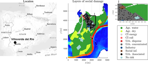
To test and illustrate the approach proposed, the town of Villaverde del Rio has been selected for a virtual case study (see Figure 2). The position of this town is just north of the Guadalquivir river, and east of another smaller river called the Arroyo de los Siete Arroyos. The flooding predictions (created using the methodologies of MAPA (2013, 2015)) for this location are presented for three return periods (10 years: T10; 100 years: T100; 500 years: T500) in the CHG Geoportal.¹

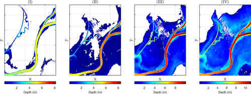
Data from this flood risk assessment supported the development of a virtual case study to research on adaptation and flood mitigation. It consists in creating scenarios with associated probability of flooding from the annual maxima event. Figure 1 presents realisations of flood depth for different probabilities. This location, and in particular this region, has been affected by recurrent flooding events (DHE, 2019) and the newly developed assessments on flood risk (driven by the EU (2007) directive) show that several locations of this region are expected to be at large risk of flooding.

Details are in the caption following the image — **FIGURE 1**
Open in figure viewer PowerPoint

The sub-figures (I) and (II) represent virtually generated depth profiles with annual exceedances of 90% and 70%; and (III) and (IV) represent the depth profiles with annual exceedance of 10% and 1% as defined by MAPA (2013, 2015).

The damage in a flooding event is obtained from the depth profiles and the methodology presented in MAPA (2013). Ten layers of risk are used to approximate the loss due to a flooding event, see Figure 2, which are used to develop different receptors of risk to be compared with the flood depth profiles and used in the representative case study generated. An example of the different receptors of risk is presented in the zoomed sub-figure (I) of Figure 2. In the case of a flooding event a receptor is activated depending on the value of water depth at a receptor location. The value allocated to each receptor is defined using the depth profiles and different threshold depth weights of damage as defined in the methodology of MAPA (2013). Total loss is achieved at 2 m of water depth, with 90% loss being at 1 m of water depth.

One of the characteristics of the region studied is its vulnerability to flooding, which can be identified in the large value and low variability of damage in between T10 and T100 presented in the flood risk assessment. The loss for a 10 year flooding event has an estimated value of 30.6 M€ with 22.0 M€, in the urban area, followed by losses of 2.37, 1.66 and 1.5 M€ in respectively, water agriculture, concentrated industry and rail CI.

In the present implementation, 37 virtual adaptation measures were defined to perform a representative study (see Table 1). These represent possible adaptation measures, and are set to be competitive in relation to damages of the T10 event as set by MAPA (2013, 2015) to illustrate the EQI analysis proposed. Each measure is applied to the receptors while uncertain events are generated to infer on net-cost estimates. Two main types of adaptation measures are considered, protection to thresholds of water depth and reduction of risk (e.g., can be representative of a subsidy or similar alternative that may reduce the impact or perception to the realisation of risk).

TABLE 1. Virtual adaptation measures (a_i) against flooding events to be implemented in the case study of Villaverde del Rio

Type	Applied to	Number measure (i)	Description	Cost implementation
I	Agriculture (water)	1–2	Flood barrier up to 1 and 2 m water depths	2.09 M€, 4.59 M€
II	Agriculture (water)	3–5	Reduction of any flood damages in 20% and 60% and 100%	1.04 M€, 2.61 M€, 12.53 M€
I	Agriculture (dry)	6–7	Flood barrier up to 1 and 2 m water depths	0.19 M€, 0.60 M€
II	Agriculture (dry)	8–10	Reduction of any flood damages in 30% and 60% and 100%	0.26 M€, 0.36 M€, 0.92 M€
I	Energy CI	11	No flood allowed regardless of water depth	0.15 M€
II	Energy CI	12	Reduction of any flood damages in 50%	0.03 M€
I	Rail CI	13–14	Flood barrier up to 1 and 2 m water depths	0.04 M€, 0.11 M€
II	Rail CI	15–16	Reduction of any flood damages in 60% and 100%	0.06 M€, 1.21
I	Disperse Urban area	17–18	Flood barrier up to 0.7 and 1 m water depths	0.01 M€, 0.04 M€
II	Disperse Urban area	19–20	Reduction of any flood damages in 50% and 100%	0.04 M€, 0.38 M€
I	Concentrated Urban area	21–22	Flood barrier up to 1 and 2 m water depths	1.05 M€, 12.34 M€
II	Concentrated Urban area	25–25	Reduction of any flood damages in 50%, 80% and 100%	0.21 M€, 1.84 M€, 28.88 M€
I	Concentrated Industry area	26–27	Flood barrier up to 1 and 2 m water depths	0.10 M€, 0.36 M€
II	Concentrated Industry area	28	Reduction of any flood damages in 100%	0.75 M€
I	Social infrastructure	29–30	Flood barrier up to 0.7 and 1.5 m water depths	0.06 M€, 0.32 M€
II	Social infrastructure	31–33	Reduction of any flood damages in 50%, 80% and 100%	0.05 M€, 0.06 M€, 0.69 M€
I	Associated Urban CI	34–35	Flood barrier up to 1 and 2 m water depths	0.24 M€, 1.0 M€
II	Associated Urban CI	36–37	Reduction of any flood damages in 50% and 100%	0.19 M€, 2.73 M€

Note: I—measures that mitigate flooding risk depending on a threshold depth that if surpassed will damage receptors; II—measures that reduce the value of risk in the flooded area.

These measures are the basis to build Φ(a, x) that transfer uncertain events into adapted estimates. Examples of Φ(a_i, x) for different adaptation measures considering x as annual probability of a net-cost are presented in Figure 3. In this case a two parameter Weibull distribution is fitted to data points collected at flooding events with annual probabilities of 1%, 10%, 50% and 90%. This is assumed to be adequate for the reference period of 10 years studied. To fit the Weibull parameters a squared error to the Φ(a_i, x) value is minimised at the four points assessed. The approximation error for model prediction in the reference points is lower than 1% for all the z_a studied. Other alternatives for fitting could use other measures of Goodness-of-fit, and four additional are discussed in Teixeira et al. (2018). The two-parameter Weibull model has wide applicability (Rinne, 2008) and support in $[0, + \infty [$ which is of interest for an application of risk that relies in estimates of damage. Nonetheless, as highlighted in Teixeira, Nogal, and O'Connor (2019), the upper unbounded threshold for the support of any transfer models may impose some limitations and needs to be accounted for. In the present, an upper bound of loss is imposed by the event that has a recurrence of 500 years (38.8 M€).

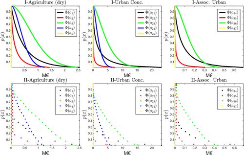
Examples of fitted curves using the four probabilities aforementioned are presented in Figure 3,I for the a_i of dry agriculture, urban concentrated areas and infrastructure associated with urban areas. These can be compared with Figure 3,II, where outcomes are modelled for 25 p(x) with different associated probability ∈ [0,1[ are presented for each respective risk layer and adaptation measure. It is possible to infer that for most a_i the transfer curves produce an efficient prediction, with exception of measure 21 and 23 in the urban concentrated where there is a slight overestimation of the value ϕ(a, x) for low probability events.

The idea of Φ is therefore to approximate any event damage by a subset x, or (p(x)), occurrences for a certain z_a decision; regardless of the number of uncertainty sources enclosed in the analysis. The relationship between uncertain events, adaptation and damage should be smooth and the same rationale is implemented in engineering analyses that use surrogates (Kay et al., 2014; Teixeira et al., 2021).

It is noted that this virtual case study is representative of adaptation to flooding that has a sense of urgency, hence, a decision that should not be further delayed.

4.1 Simulation of a T period

Monte–Carlo simulation (MCS) is applied to simulate annual events to research a reference period T of 10 years. MCS is commonly found in the study of flood adaptation (Simonović, 2012). It does not depend on any assumptions of the problem being addressed, and its combination with Φ(z_a, x) enables to relate occurrences, their probability, with the outcome from adaptation. To assess event variability, a MCS sample comprises n vectors of T probabilities that translate to a set of x, and that feed an analysis with Φ(a, x).

The empirical cumulative distribution function from MCS for three scenarios over a 10 year period are presented in Figure 4. Figure 4a considers only the aleatory uncertainty of annual events. Considering that each 10 years random occurrence of events represents a probabilistic combination of x for this region, then z_a optimal ad-hoc x represents the case where for each 10 years random occurrence it would be possible to choose the optimal ad-hoc z_a decisions according to Equation (4). This is not possible in the present as it would imply a capability to adapt in a tailored format if exact predictions could be made. Therefore, the optimal z_a∀x represents the z_a decision that minimises the total net-cost over the probabilistic combinations of events.

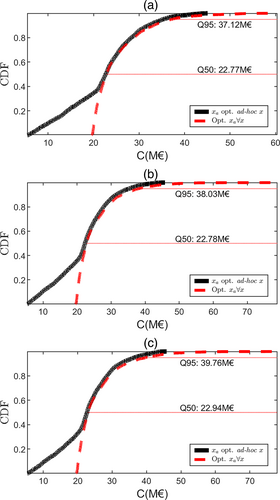
Figure 4b considers also that the risk assessment for each layer is uncertain following a Gaussian distribution with a coefficient of variation of 20% and mean equal to the current estimation. In this case an uncertain x is a combination of probability of flooding event with that of a risk deviation. This uncertainty in the risk assessment as used in this reference example is easily included in Φ(a, x). It can be introduced in the transfer function as defined through the estimation of the fitted Φ(a, x) without additional need of additional x evaluations; however, demanding the Weibull model to be re-tuned for the risk value. Figure 4c considers the sources of uncertainty in (a) and (b) and that in the following 10 years there is also a 20% chance of an increase of maxima occurrences of 10%, a 15% chance of an increase of maxima occurrences of 20%, and a 65% probability of no increase in maxima occurrences.

One particular finding arising from the analysis of (a, b, c) is that while the inclusion of the probabilistic character of the assessment has a smaller influence over the expected value (to some extent understandable due to the relationship of the assumptions with the expected value), there is a significant change in the tail of the distribution with the maximum C(z_a, x, T) increasing almost 25% in (b) and (c) when compared with (a) for the sample size studied. In relation to expected values, this is equivalent to an increase of approximately 100% of C(z_a, x, T) (that are in (a) ≈ 24.5 M€, in (b) ≈ 25.1 M€ and in (c) ≈ 25.5 M€).

Quantiles for the 50%(Q50) and 95%(Q95) of data in the empirical cumulative distribution are also presented in Figure 4. It is possible to infer that the increase in Q50 and Q95 is more pronounced from 1 to 2. The fact that Q50 is lower than the average, indicates that there is a long tail in this distribution. The analysis of Q95 shows an increase of approximately 50% to the mean in all the three cases, which is a relatively high probability of surpassing the expected value of the total cost in 50%.

The discussion of probabilistic output from adaptation highlights that there is interest in researching from both the perspective of expectation and some form of guaranteed protection. This forms the foundation of an EQI evaluation.

4.2 Expectation–quantile and its relevance

An analysis of expectation and quantiles is now performed, first with discussion of the relevance of assessing the probabilistic outcomes from adaptation. Modelling conditions are the same as applied in (c) in the previous section.

A genetic algorithm (GA) is used to solve the multiple objective optimization to find the optimal z_a. Simonović (2012) provides an overview of the usage of GA in flood adaptation and Teixeira et al. (2022) discuss its application in the context of enabling adaption that considers uncertainty. The dependence of f_Q(z_a, x) on the full distribution function and MCS to define the quantile of interest increases the complexity and effort necessary to set this evauation as a linear optimization problem. It is noted that as z_a is integer, the Pareto frontier is non-continuous.

Figure 5 presents the Pareto front for the E–Q considering a quantile of 99% and 99.9%. Both represent a high confidence of protection for a period of 10 years. This is the case of analysing the balance between expectation of net-cost and the confidence on a maximum protection.

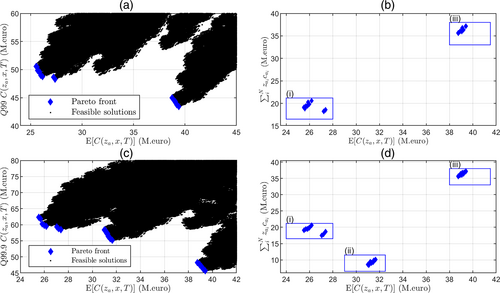
In the context of E–Q optimality solutions cluster in two main regions for Q99 (i and iii) in Figure 5a,b and three for Q99.9 (i, ii and iii) in Figure 5c,d, being (i) a region of low expectation and large quantile net-cost, (ii) a balanced region in terms of expectation and quantile and (iii) a region of large expected net-cost and lower maximum net-cost. An interesting outcome of the present analysis is the realisation of a balanced region of relatively low investment that offers a balanced trade-off in quantile and expected cost, and that shows in Q99.9. This region is represented by the cluster of points in Figure 5d with an investment of approximately 9.5 M€ and expected net-cost of approximately 31.5 M€—region (ii).

The cumulative distribution functions of C(z_a, x, T) for the three solutions in the regions (i), (ii) and (iii) in the case of (c,d) are presented in Figure 6. These include the solutions that minimise the quantile (min Q [C(z_a, x)]), the expectation ( $\min E [C (z_{a}, x)$ ]) and the investment ( $\min \sum_{i}^{N} z_{a_{i}} c_{a_{i}}$ ). The solution that minimises the expectation requires an investment of 19.0 M€. The solution that offers a balanced trade-off at a minimum investment requires 9.37 M€. Finally the adaptation that minimises the loss at the quantile studied requires 37.39 M€.

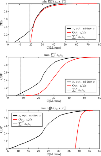
In terms of expectation of net-cost, the first has an expected C(z_a, x) of 25.53 M€, the second 31.09 M€ and the third 39.56 M€. The main difference between these decisions of adaptation is fundamentally centred in the approach to protect the concentrated urban areas (measures 21, 24 and 25), where most of the costs will be incurred in the case a flooding event reaches the area, see Figure 7. Measure 21 offers protection to the urban concentrated area, however, there is a probability of it failing (being overtopped), and even considering its low likelihood, if it occurs the damages to urban concentrated areas are significant. In the solution that has lower investment, $\min \sum_{i}^{N} z_{a_{i}} c_{a_{i}}$ , this measure is replaced by an alternative that is equivalent to reducing the perception of the risk in 80% of its realisation. This measure, less expensive as defined, allows for overall higher distribution risk realisation.

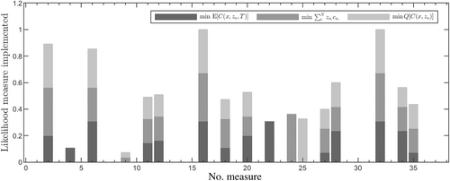
It is interesting to note that the investment decision with lowest $\sum_{i}^{N} z_{a_{i}} c_{a_{i}}$ provides the largest ratio of euro saved per invested. However, when compared with the case of $\min E [C (z_{a}, x, T)]$ , while it produces greater gains at a lowest value (with a decrease of ~9.63 M€), in objective terms it has an expected value of C(z_a, x, T) that is 5.5 M€ larger. As a result there is a large likelihood of experiencing ~51.4% of this reduction in investment in flood loss. This generates the question to whether an additional effort should be put in place to invest instead of accepting risk. Moreover, realisation of the risk may potentiate additional unforeseen loss.

This analysis emphasises the ways in which being able to address uncertainty and different criteria in decision-making is informative, in particular combining budget with outcomes. This will be further discussed in the application of EQI decisions.

4.2.1 EQI optimal decisions

If most decision-making in adaptation needs to deal with a budget for investment and such large discrepancies can be found in the probabilistic outcomes of adaptation for different investments, it can be argued that an objective unrestrained analysis (in budget) is valuable to understand the outcomes of investment decisions considering also the uncertainty in the outcomes of other variables. This is the main rationale of a EQI evaluation. Q99 are applied as a practical reasonably low risk criteria for accepting a quantile event and Figure 8 presents the results for an EQI evaluation of the presented example in the previous section.

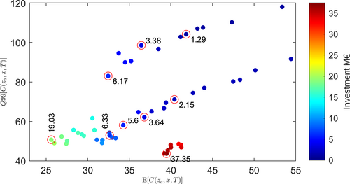
In a context of optimal decisions, the EQI allows to infer that if decision-making is centred on minimising a decision to an occurrence or an expected scenario in a spectra of occurrences then, from a probabilistic perspective (that of selecting an expectation that is also robust in terms of not experiencing a large maxima), this may lead to a decision that is only efficient in expected value. Figure 8 shows that adaptation decisions that are competitive in $E [C (z_{a}, x, T)]$ may not be in terms of Q[C(z_a, x, T)], and this may lead to the selection of measures that are not competitive regarding the risk of large failures (in this case with a 1% exceedance chance) for a pre-specified budget. It is therefore relevant to have different optimal points in this triaxial competitive criteria.

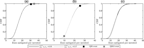
This is particularly evident in points highlighted that have similar budget but significant differences in Q99. Examples are found in the investment of 6.33 and 6.17 M€, or 3.64 and 3.38 M€. It is also evident when solutions with progressively larger investment are considered, and where a small adjustment of the investment can bring significant gains in terms of the overall probabilistic outcome of adaptation. The EQI allows to map optimality in the additional effort of investment with the gains in expectation, and potential deviations from it. This is particularly relevant when multiple possibilities of adaptation exist, which may be pose a challenge for decision-making schemes. Furthermore, it allows to identify outcomes of simple variations of budget that may lead to significant differences in probabilistic outcomes. The previous highlighted cases show that a simple addition of investment may allow to decrease the quantile at 99% by approximately 30%. In the particular case of an investment of 6.33 and 6.17 M€, 89% of the increase in expectation of net-cost is due to the additional investment of 0.16 M€, however, the result of this investment is a reduction of the Q99 net-cost in 30.2 M€. For this case, the ratios of euro mitigated per invested have the empirical distribution forms presented in Figure 9. While this ratio is larger over most of the empirical CDF for the solution with investment of 6.17 M€, the ratio for the event that originates the quantile 99% and 99.9% C(z_a, x, T) is smaller and appears earlier in its empirical CDF (see Figure 9a,b). That is, even considering the lower investment and the overall distribution offering a larger ratio for most of the empirical cumulative density function, in the specifically damaging events this decision does not perform as well and the benefit per euro invested is smaller (see Figure 9c).

The overall achievement of an EQI analysis is that it is more informative with respect to the uncertainties that affect the decision-making scheme for flooding events; which allows decisions based on three dimensions that will have large influence on the performance of the adaptation implemented. The discussed example remarks how probabilistic outcomes can be highly affected by small margins when investment is considered. It shows the solutions in this tridimensional analysis that dominate all the other alternatives. And while a sensitivity analysis may allow to identify similar patterns, it is effort-consuming when multiple adaptation options are available and may fail to enclose the solutions that are not dominated by other feasible choice and that have the most interest in terms of efficiency of the implementation.

4.2.2 Beyond EQI optimality

It is of interest in future works to further elaborate on time considerations used in the approach developed to infer on the influence of the time when the adaptation z_a is implemented, and as such, weight on the benefit and risk of holding the investment. Under a EQI analysis these can be considered, and transfer functions can be also applied for this effect. Manocha and Babovic (2018) combine real options with a multiobjective optimization under a dynamic pathways analysis. A similar approach can be undertaken with EQI decisions and evaluation of uncertainties, including deep uncertainties, to show the optimality trade-off of investment and benefits for different pathways.

It is also noted that flood adaptation is expected to consider more than monetary terms of damage and resource consumption. Different uncertainties that in practice cannot be explicitly monetised may need to be considered in the analysis. New objectives may be defined for that effect and included in an EQI analysis. Additionally, concepts of adaption in future works may include innovative ideas that have been exploited recently in the context of flood management, such as that of antifragility, or adaptation that enhances system operation with exposure to unfavourable conditions (Babovic et al., 2018).

5 CONCLUSION

The present work discussed an approach for flood adaptation decisions that includes its probabilistic character in the establishment of optimal decisions. It consists of finding an optimal decision for probabilistic outcomes that considers a balance of expectation, with probability confidence and levels of investment. It seems particularly important to include the probabilistic outcome of adaptation decisions in adaptation strategies at highly vulnerable locations where large deviations from expectation may occur in relatively short time-frames.

To reduce the amount of effort needed to perform a probabilistic assessment, probability curves are applied as transfer curves for adaptation. A mathematical programming problem that uses these was proposed. It is noted that with transfer curves it is possible to approximate a full probabilistic analysis using only a subset of probability events, which allows then to perform simulation at virtually no cost. The probability curves are applied with MCS in a research of an EQI analysis. This EQI enables to map optimality in a tri-dimensional axis of interest for probabilistic considerations (i.e., expected value, probability quantiles and amount of investment). It also allows to identify relevant considerations of decision-making for adaptation, such as, the fact that in a decision-making scheme large variations in the confidence at a certain level may occur for similarly competitive decisions in terms of budget or investment and expected value of net-costs.

This triaxial approach to decisions is informative and introduces new considerations to decision-making schemes. Results from a virtual case study show that marginally different and equally competitive alternatives in terms of investment and expected net-costs may have probabilistic deviations of extreme occurrences of over 30% in relation to the larger value (or 54% in relation to the minor value).

Approaches that include probabilistic information, other than the expected value, will have progressively more importance in the future as decisions need to be informed in regard to potential outcomes from the different uncertainties that affect these. Future works should investigate the effects of time varying decision characteristics (holding investment) in the period of reference and on their incorporation in the analysis proposed. Extension of this approach to address uncertainties that cannot be explicitly considered is also of interest, such as the case of imprecise probabilities or deep uncertainties.

ACKNOWLEDGEMENTS

This work was supported by the Interreg [EAPA 45/2018-AAFLOODS Project]. Open access funding provided by IReL.

ENDNOTE

¹ https://idechg.chguadalquivir.es/nodo/index.html

Open Research

DATA AVAILABILITY STATEMENT

The data that support the findings of this study are available from the corresponding author upon request.

REFERENCES

Abadie, L. M., de Murieta, E. S., & Galarraga, I. (2017). Investing in adaptation: Flood risk and real option application to Bilbao. Environmental Modelling & Software, 95, 76–89.
10.1016/j.envsoft.2017.03.038
Web of Science® Google Scholar
Apel, H., Thieken, A. H., Merz, B., & Blöschl, G. (2006). A probabilistic modelling system for assessing flood risks. Natural Hazards, 38(1), 79–100.
10.1007/s11069-005-8603-7
Web of Science® Google Scholar
Arias, P., Bellouin, N., Coppola, E., Jones, R., Krinner, G., Marotzke, J., Naik, V., Palmer, M., Plattner, G.-K., Rogelj, J., Rojas, M., Sillmann, J., Storelvmo, T., Thorne, P. W., Trewin, B., Rao, K. A., Adhikary, B., Allan, R. P., Armour, K., … Zickfeld, K. (2021). 2021: Technical summary. In V. Masson-Delmotte, P. Zhai, A. Pirani, S. L. Connors, C. Péan, S. Berger, N. Caud, Y. Chen, L. Goldfarb, M. I. Gomis, M. Huang, K. Leitzell, E. Lonnoy, J. B. R. Matthews, T. K. Maycock, T. Waterfield, O. Yelekçi, R. Yu, & B. Zhou (Eds.), Climate change 2021: The physical science basis. Contribution of working group14 I to the sixth assessment report of the intergovernmental panel on climate change. Cambridge University Press.
Google Scholar
Babovic, F., Babovic, V., & Mijic, A. (2018). Antifragility and the development of urban water infrastructure. International Journal of Water Resources Development, 34(4), 499–509.
10.1080/07900627.2017.1369866
Web of Science® Google Scholar
Buurman, J., & Babovic, V. (2016). Adaptation pathways and real options analysis: An approach to deep uncertainty in climate change adaptation policies. Policy and Society, 35(2), 137–150.
10.1016/j.polsoc.2016.05.002
Web of Science® Google Scholar
Castillo, E. (2012). Extreme value theory in engineering. Elsevier.
Google Scholar
Chang, M.-S., Tseng, Y.-L., & Chen, J.-W. (2007). A scenario planning approach for the flood emergency logistics preparation problem under uncertainty. Transportation Research Part E: Logistics and Transportation Review, 43(6), 737–754.
10.1016/j.tre.2006.10.013
Web of Science® Google Scholar
De Neufville, R., & Scholtes, S. (2011). Flexibility in engineering design. MIT Press.
10.7551/mitpress/8292.001.0001
Google Scholar
Deng, Y., Cardin, M.-A., Babovic, V., Santhanakrishnan, D., Schmitter, P., & Meshgi, A. (2013). Valuing flexibilities in the design of urban water management systems. Water Research, 47(20), 7162–7174.
10.1016/j.watres.2013.09.064
CAS PubMed Web of Science® Google Scholar
DHE. (2019). Revisión y actualización de la evaluación preliminar del riesgo de inundación. Demarcación Hidrográfica del Guadalquivir.
Google Scholar
Dittrich, R., Ball, T., Wreford, A., Moran, D., & Spray, C. J. (2019). A cost-benefit analysis of afforestation as a climate change adaptation measure to reduce flood risk. Journal of Flood Risk Management, 12(4), e12482.
10.1111/jfr3.12482
Web of Science® Google Scholar
Dottori, F., Mentaschi, L., Bianchi, A., Alfieri, L., & Feyen, L. (2020). Adapting to rising river flood risk in the eu under climate change (p. 14505). Publications Office of the European Union.
Google Scholar
European Commission. (2007). EU directive 2007/60/EC: On the assessment and management of flood riks. Technical report. European Commission.
Google Scholar
Garrido, R. A., Lamas, P., & Pino, F. J. (2015). A stochastic programming approach for floods emergency logistics. Transportation Research Part E: Logistics and Transportation Review, 75, 18–31.
10.1016/j.tre.2014.12.002
Web of Science® Google Scholar
Haasnoot, M., Kwakkel, J. H., Walker, W. E., & Ter Maat, J. (2013). Dynamic adaptive policy pathways: A method for crafting robust decisions for a deeply uncertain world. Global Environmental Change, 23(2), 485–498.
10.1016/j.gloenvcha.2012.12.006
Web of Science® Google Scholar
Hall, J., & Solomatine, D. (2008). A framework for uncertainty analysis in flood risk management decisions. International Journal of River Basin Management, 6(2), 85–98.
10.1080/15715124.2008.9635339
Google Scholar
Helmrich, A. M., & Chester, M. V. (2022). Reconciling complexity and deep uncertainty in infrastructure design for climate adaptation. Sustainable and Resilient Infrastructure, 7(2), 83–99.
10.1080/23789689.2019.1708179
Web of Science® Google Scholar
Jha, A. K., Bloch, R., & Lamond, J. (2012). Cities and flooding: A guide to integrated urban flood risk management for the 21st century. World Bank Publications.
10.1596/978-0-8213-8866-2
Google Scholar
Jongman, B. (2018). Effective adaptation to rising flood risk. Nature Communications, 9(1), 1–3.
10.1038/s41467-018-04396-1
CAS PubMed Web of Science® Google Scholar
Jongman, B., Ward, P. J., & Aerts, J. C. (2012). Global exposure to river and coastal flooding: Long term trends and changes. Global Environmental Change, 22(4), 823–835.
10.1016/j.gloenvcha.2012.07.004
Web of Science® Google Scholar
Jung, Y., & Merwade, V. (2012). Uncertainty quantification in flood inundation mapping using generalized likelihood uncertainty estimate and sensitivity analysis. Journal of Hydrologic Engineering, 17(4), 507–520.
10.1061/(ASCE)HE.1943-5584.0000476
Web of Science® Google Scholar
Kay, A. L., Crooks, S. M., Davies, H. N., Prudhomme, C., & Reynard, N. S. (2014). Probabilistic impacts of climate change on flood frequency using response surfaces i: England and Wales. Regional Environmental Change, 14(3), 1215–1227.
10.1007/s10113-013-0563-y
Web of Science® Google Scholar
Kheradmand, S., Seidou, O., Konte, D., & Batoure, M. (2018). Evaluation of adaptation options to flood risk in a probabilistic framework. Journal of Hydrology: Regional Studies, 19, 1–16.
10.1016/j.ejrh.2018.07.001
Web of Science® Google Scholar
Kull, D., Mechler, R., & Hochrainer-Stigler, S. (2013). Probabilistic cost-benefit analysis of disaster risk management in a development context. Disasters, 37(3), 374–400.
10.1111/disa.12002
CAS PubMed Web of Science® Google Scholar
Lasage, R., Veldkamp, T., De Moel, H., Van, T., Phi, H., Vellinga, P., & Aerts, J. (2014). Assessment of the effectiveness of flood adaptation strategies for hcmc. Natural Hazards and Earth System Sciences, 14(6), 1441–1457.
10.5194/nhess-14-1441-2014
Web of Science® Google Scholar
Lendering, K. T., Sebastian, A., Jonkman, S. N., & Kok, M. (2019). Framework for assessing the performance of flood adaptation innovations using a risk-based approach. Journal of Flood Risk Management, 12(S2), e12485.
10.1111/jfr3.12485
Web of Science® Google Scholar
Lorie, M., Neumann, J. E., Sarofim, M. C., Jones, R., Horton, R. M., Kopp, R. E., Fant, C., Wobus, C., Martinich, J., O'Grady, M., & Gentile, L. E. (2020). Modeling coastal flood risk and adaptation response under future climate conditions. Climate Risk Management, 29, 100233.
10.1016/j.crm.2020.100233
PubMed Web of Science® Google Scholar
Manocha, N., & Babovic, V. (2017). Development and valuation of adaptation pathways for storm water management infrastructure. Environmental Science & Policy, 77, 86–97.
10.1016/j.envsci.2017.08.001
Web of Science® Google Scholar
Manocha, N., & Babovic, V. (2018). Real options, multi-objective optimization and the development of dynamically robust adaptive pathways. Environmental Science & Policy, 90, 11–18.
10.1016/j.envsci.2018.09.012
Web of Science® Google Scholar
MAPA. (2013). Propuesta de mínimos para la metodología de realización de los mapas de riesgo de inundación. Technical report. Ministerio de Agricultura, Pesca y Alimentación.
Google Scholar
MAPA. (2015). Sistema nacional de cartografia de zonas inundables mapas de peligrosidad y riesgo demarcación hidrográfica del guadalquivir. Technical report. Ministerio de Agricultura,Pesca y Alimentación.
Google Scholar
Morrison, A., Westbrook, C. J., & Noble, B. F. (2018). A review of the flood risk management governance and resilience literature. Journal of Flood Risk Management, 11(3), 291–304.
10.1111/jfr3.12315
Web of Science® Google Scholar
Muis, S., Güneralp, B., Jongman, B., Aerts, J. C., & Ward, P. J. (2015). Flood risk and adaptation strategies under climate change and urban expansion: A probabilistic analysis using global data. Science of the Total Environment, 538, 445–457.
10.1016/j.scitotenv.2015.08.068
CAS PubMed Web of Science® Google Scholar
Rehman, S., Sahana, M., Hong, H., Sajjad, H., & Ahmed, B. B. (2019). A systematic review on approaches and methods used for flood vulnerability assessment: Framework for future research. Natural Hazards, 96(2), 975–998.
10.1007/s11069-018-03567-z
Web of Science® Google Scholar
Rinne, H. (2008). The Weibull distribution: A handbook. Chapman and Hall/CRC.
10.1201/9781420087444
Google Scholar
Salman, A. M., & Li, Y. (2018). Flood risk assessment, future trend modeling, and risk communication: A review of ongoing research. Natural Hazards Review, 19(3), 04018011.
10.1061/(ASCE)NH.1527-6996.0000294
Web of Science® Google Scholar
Simonović, S. P. (2012). Floods in a changing climate: Risk management. Cambridge University Press.
10.1017/CBO9781139088404
Google Scholar
Teixeira, R., Nogal, M., & O'Connor, A. (2018). On the suitability of the generalized pareto to model extreme waves. Journal of Hydraulic Research, 56(6), 755–770.
10.1080/00221686.2017.1402829
Web of Science® Google Scholar
Teixeira, R., Nogal, M., & O'Connor, A. (2019). Analysis of long-term loading characterization for stress-cycle fatigue design. Wind Energy, 22(11), 1563–1580.
10.1002/we.2389
Web of Science® Google Scholar
Teixeira, R., O'Connor, A., & Nogal, M. (2019). Probabilistic sensitivity analysis of offshore wind turbines using a transformed kullback-leibler divergence. Structural Safety, 81, 101860.
10.1016/j.strusafe.2019.03.007
Web of Science® Google Scholar
Teixeira, R., Martinez-Pastor, B., Nogal, M., & O'Connor, A. (2021). Reliability analysis using a multi-metamodel complement-basis approach. Reliability Engineering & System Safety, 205, 107248.
10.1016/j.ress.2020.107248
Web of Science® Google Scholar
Teixeira, R., Martinez-Pastor, B., Nogal, M., & O'Connor, A. (2022). Metamodel-based metaheuristics in optimal responsive adaptation and recovery of traffic networks. Sustainable and Resilient Infrastructure, 7(6), 756–774.
10.1080/23789689.2022.2029325
Web of Science® Google Scholar
Vanneuville, W., Wolters, H., Scholz, M., Werner, B., & Uhel, R. (2016). Flood risks and environmental vulnerability: Exploring the synergies between floodplain restoration, water policies and thematic policies. EEA Report.
Google Scholar
Wagenaar, D., Dahm, R., Diermanse, F., Dias, W., Dissanayake, D., Vajja, H., Gehrels, J., & Bouwer, L. (2019). Evaluating adaptation measures for reducing flood risk: A case study in the city of Colombo, Sri Lanka. International Journal of Disaster Risk Reduction, 37, 101162.
10.1016/j.ijdrr.2019.101162
Web of Science® Google Scholar

Volume16, Issue1

March 2023

e12875

Flood adaptation decision-making for vulnerable locations using expectation–quantile–investment analysis

Abstract

1 INTRODUCTION

2 ADAPTATION TO FLOODING USING A PROBABILISTIC ANALYSIS

3 OPTIMAL PROBABILISTIC ADAPTATION TO FLOODING

3.1 Application of probability transfer functions