Climate change impacts on flood peaks in Britain for a range of global mean surface temperature changes
Funding information: The Climate Change Committee (CCC)
Abstract
An increase in extreme weather events is leading to increased flood occurrence and risk in many areas. Although climate mitigation strategies are being implemented, it is widely accepted that societies must adapt to climate variability and climate change. Traditional climate change impact studies have used projections for future time-slices, often for a range of possible emissions scenarios. Recently however, there has been a move to instead consider climate change impacts relative to global mean surface temperature (GMST) change, to try to encourage action to avoid the more severe impacts from higher GMST changes. To support adaptation planning, more localised information on impacts is required. Here, data on the potential range of changes in flood peaks is generated by combining flood response surfaces and the new UK Climate Projections 2018, for every river cell on a 1 km grid across Britain, for GMST changes of 1–4.5°C. The results show significant spatial variation, with impacts typically higher in the west than the east, and generally increasing with GMST change. Some southern regions show flood peak changes accelerating with GMST change. The changes in flood peaks can be translated into changes in flood inundation and associated flood risk under alternative adaptation assumptions.
1 INTRODUCTION
Floods impact people and the economy. Using 50 years of European river flow records Blöschl et al. (2019) concluded that observed flood changes were generally consistent with climate model projections for the next century, and that climate-driven changes are already observable within the flow record. Studies using future projections have shown that climate change is likely to affect flood occurrence globally (Arnell & Gosling, 2016; Hirabayashi et al., 2013), and when combined with socioeconomic growth significantly increase risk (Winsemius et al., 2015).
The Paris Agreement of 2015 set out to limit global mean surface temperature (GMST) change, from pre-industrial levels, to well below 2°C, whilst actively pursuing efforts to limit it to below 1.5°C (UNFCCC, 2015). Since then, scientists have been investigating how an increase in GMST of 1.5°C or more could impact natural and human systems (Hoegh-Guldberg et al., 2018). The IPCC Special Report on Global Warming of 1.5°C (IPCC, 2018) found, with high confidence, that the increase in GMST (which reached 0.87°C in 2006–2015 relative to 1850–1900) has increased the frequency and magnitude of impacts such as temperature and precipitation extremes, leading to changes in drought, flooding, food security and human health. Using the HAPPI protocol (Half a degree Additional warming, Prognosis and Projected Impacts; Mitchell et al., 2017) to generate an ensemble of simulations, Paltan et al. (2018) found that global historical 100-year return period floods occur more frequently at 1.5°C, but even greater additional changes are projected for regions such as South America, central Africa and central-Western Europe at 2°C. At the continental scale, for a multi-model study in Europe, Alfieri et al. (2018) report that global warming is linked to a substantial increase in flood risk over most countries in Central and Western Europe at all warming levels (1.5, 2 and 3°C). Considering European river high flows (10% exceedance probability of streamflow) and floods (annual maximum), Thober et al. (2018) found projected decreases in both high flows (up to −31% at 3°C warming) and floods (up to −17% at 3°C warming) in the Mediterranean and Eastern Europe mostly related to decreases in total annual precipitation. In Northern regions they found that, for GMST changes of 1.5, 2 and 3°C, high flows are projected to increase due to increasing precipitation but decreases in snowmelt lead to a projected decrease in floods.
River basin studies such as Huang et al. (2018) show that regional effects of specific warming levels are necessary to provide more detailed estimates of potential changes. Liu et al. (2017) found that the Yiluo river catchment in Northern China is projected to have more significant changes in 25- and 50-year return period floods than the Beijiang river (Southern China). The mean annual runoff for the Yilou is projected to decrease by 22 and 21% for GMST changes of 1.5 and 2°C, respectively, whereas for the Beijiang the mean annual runoff is projected to increase by less than 1 and 3% for GMST changes of 1.5 and 2°C. In the Ganges-Brahmaputra-Meghna basin, Uhe et al. (2019) reported enhanced flood risk at 1.5 and 2°C warming with small differences in changes of flooded area for the three sub-basins. The relative change in flood area decreases for the 1 in 20 and 1 in 100 year floods, and the less frequent (more severe) 1 in 100 year flood area in the Ganges and Brahmaputra rivers show a smaller change than the relative precipitation change.
Traditionally, climate model data have been used to drive impact models (e.g., Arheimer & Lindström, 2015; Bell et al., 2016; Fiseha et al., 2014). However, other techniques have been adopted based on a sensitivity domain approach (e.g., Wetterhall et al., 2011), which negate the need to repeat modelling studies whenever new climate projections are released. Such an approach typically involves running a set of sensitivity experiments and producing so-called response surfaces. The response surfaces represent the sensitivity of an impact measure to a set of plausible climatic changes; sets of climate projections can then be overlaid on the response surfaces to estimate future impacts.
Prudhomme et al. (2010) developed a sensitivity framework for estimating the impacts of climate change on peak flows in Great Britain (GB). This was applied with the probabilistic projections from UKCP09 (Murphy et al., 2009) to assess the potential range of impacts of climate change on flood peaks on a regional basis (Kay, Crooks, Davies, Prudhomme, Reynard, 2014; Kay, Crooks, Davies, & Reynard, 2014). Recently, Kay et al. (2021) used the sensitivity framework approach with a national-scale grid-based hydrological model to produce flood response surfaces for 1 km grid boxes across GB, enabling consistent assessment of sensitivity for catchments across GB (gauged or ungauged). The authors then applied the new probabilistic projections from UKCP18 (Lowe et al., 2018), by overlaying them on the modelled response surfaces, to assess the potential impacts of climate change on flood peaks across the whole country, for a range of future time-slices and emissions scenarios.
- deriving sets of UKCP18 probabilistic projections for each of the required GMST changes (1°C to 4.5°C in increments of 0.5°C);
- overlaying the sets of projections on the modelled response surfaces from Kay et al. (2021);
- developing a way of correcting for the effect of incomplete probabilistic samples for higher GMST changes (3°C and over).
Investigating flood peak changes across GB relative to levels of GMST change, rather than by future time-slice and emission scenario as done previously, directly illustrates the additional impact that higher levels of GMST change could have, regardless of when the level is reached or what emissions trajectory is taken to get there. This form of climate change impacts analysis thus fits better with the current focus of national and global policy on climate change—to limit global warming to below certain thresholds. The methods are described in Section 2, with results in Section 3, discussion in Section 4 and conclusions in Section 5.
2 METHODS
2.1 The sensitivity-based method for estimating changes in peak river flows
2.1.1 Background
Sensitivity-based methods can be used to generate ‘response surfaces’, which illustrate estimated changes in a variable of interest under a broad set of plausible climatic changes. This study uses the two-dimensional (2D) flood response surfaces produced by Kay et al. (2021), who applied the sensitivity-based method of Prudhomme et al. (2010) with the Grid-to-Grid national-scale grid-based hydrological model (G2G; Bell et al., 2009) to estimate changes in peak river flows across GB for a range of future time-slices and emissions scenarios.
Full details of the method used to produce the flood response surfaces are provided by Kay et al. (2021). Briefly, following Prudhomme et al. (2010), the monthly pattern of precipitation changes was assumed to take the form of a harmonic function with the peak in January; X0 + A cos [2π (t − 1)/12], for month t, annual mean change X0 and amplitude A. This gives precipitation changes of X0 + A in January (t = 1), X0 − A in July (t = 7), and smooth variation between these values for the intervening months. X0 was varied in 5% increments from −40 to +60% (21 values), and A was varied in 5% increments from 0 to 120% (25 values). X0 and A thus form the two dimensions of the response surface, representing a total of 525 (21 × 25) sets of changes in precipitation. A small set of alternative scenarios for changes in temperature, and corresponding changes in potential evaporation (PE), were applied alongside the precipitation changes, forming alternative response surfaces. The sets of monthly climatic changes were applied to baseline climate time-series using the change factor method (sometimes called the delta change method, e.g., Arnell et al., 2020, Kay et al., 2020), to provide adjusted driving climate data for the model. Each square on the 2D flood response surface represents the results of a hydrological model run driven by one set of climatic changes (precipitation and temperature/PE), and is coloured according to the corresponding modelled change in peak river flow (for 10-, 20- or 50-year return periods) (see Kay et al. (2021) Figure 1 for example flood response surfaces).

Kay et al. (2021) produced modelled flood response surfaces for all non-tidal river cells on a 1 km grid (with catchment area ≥100 km2); a total of 12,421 1 km river cells, across 19 river-basin regions (Supplementary Section 1.1). Only the response surfaces for 50-year return period peak flows and for the main temperature/PE scenario (termed medium-August) are used here.
2.1.2 Flood response types and representative flood response surfaces
Prudhomme et al. (2013) used the flood responses surfaces generated for 154 catchments to identify nine flood response types, each with representative flood response surfaces (Figure 1). These characterise the range of differing catchment sensitivity to climatic change. Catchments with a Neutral response type show changes in peak flows similar to the changes in precipitation. Catchments with a Damped type (Damped-Extreme, Damped-High, Damped-Low) show peak flow changes generally smaller than the precipitation changes, and those with an Enhanced type (Enhanced-Low, Enhanced-Medium, Enhanced-High) show peak flow changes that are often larger than the precipitation changes. For catchments with Mixed or Sensitive types, the peak flow changes are more variable, depending on the seasonality and magnitude of the changes in precipitation.
Kay, Crooks, and Reynard (2014) assessed the uncertainty from the assumptions/simplifications necessary to develop/implement the sensitivity-based approach, which led to the generation and application of extra uncertainty allowances for each response type. Kay et al. (2021) compared the modelled response surfaces for each 1 km river cell with the representative flood response surfaces (Figure 1) to generate 1 km grids of the best-matching response type. As in Kay et al. (2021), these are used to apply the extra uncertainty allowances here. They are also used when correcting for the effect of incomplete probabilistic samples for higher GMST changes (Section 2.4).
2.2 The UKPC18 probabilistic projections
UKCP18 provides probabilistic projections, consisting of 3000 sets of changes in a number of climate variables, on a 25 km grid or for river-basin regions (Supplementary Section 1.1), for four Representative Concentration Pathways (RCP2.6, 4.5, 6.0, 8.5; van Vuuren et al., 2011). Kay et al. (2021) overlaid the sets of river-basin region probabilistic projections on the 1 km modelled flood response surfaces, to estimate projected changes in peak river flows for three future 30-year time-slices (2020s, 2050s and 2080s, relative to 1961–1990) under each of the four RCPs.
Here though, it is necessary to select different future time-slices for each of the 3000 ensemble members within the probabilistic projections, corresponding to each required GMST change (Section 2.2.1). Corresponding precipitation changes are then derived (Section 2.2.2) and overlaid on the modelled response surfaces of Kay et al. (2021), to determine projected changes in peak river flows for specific GMST changes (Section 2.3). However, not all of the 3000 probabilistic ensemble members reach all of the required GMST changes by 2100. Thus, it is necessary to develop a way of correcting for the effect of incomplete ensembles (Section 2.4).
2.2.1 GMST changes and time-slice selection
Available with the UKCP18 Probabilistic projection data are yearly GMST anomalies (°C, relative to the baseline period 1981–2000) for each ensemble member (December 1859–November 2099; Supplementary Section 1.2). These are used to derive sets of probabilistic projections corresponding to specific GMST changes, as described below. The probabilistic projection data for RCP8.5 are used for all of the required GMST changes, as this high RCP is the one covering the greatest range of GMST changes.
The yearly GMST anomalies are turned into time-slice mean changes for all possible future 20-year time-slices (1971–1990, 1972–1991, …, 2080–2099) from an alternative (pre-industrial) baseline (1860–1900) (Supplementary Section 1.2.1). For each required GMST change and each ensemble member, the time-slice with mean GMST change closest to the required GMST change is identified (within a maximum deviation of 0.04999°C). Supplementary Table 1 shows an example of this time-slice selection for a subset of seven ensemble members.
Note that not all required GMST changes have a full set of 3000 samples (Table 1 and Supplementary Figure 4), as not all ensemble members reach each required GMST change. For this reason, the analysis could not go beyond a 4.5°C GMST change, since over 50% of the 3000 ensemble members are missing for higher GMST changes (Table 1).
| GMST change (°C from pre-industrial) | Number of ensemble members (RCP8.5) | % of missing ensemble members |
|---|---|---|
| 1.0 | 3000 | 0.0 |
| 1.5 | 3000 | 0.0 |
| 2.0 | 3000 | 0.0 |
| 2.5 | 2997 | 0.1 |
| 3.0 | 2919 | 2.7 |
| 3.5 | 2700 | 10.0 |
| 4.0 | 2213 | 26.2 |
| 4.5 | 1578 | 47.4 |
| 5.0 | 989 | 67.0 |
| 5.5 | 515 | 82.8 |
| 6.0 | 213 | 92.9 |
- Note: The Significance of Bold values indicates the corresponding % of missing ensemble members for which a correction grid has been created. Abbreviation: GMST, global mean surface temperature.
2.2.2 Precipitation changes
Sets of precipitation changes are required for each GMST change, for each selected ensemble member/time-slice combination (Section 2.2.1). These are calculated from the UKCP18 Probabilistic projections for river-basin regions (Met Office Hadley Centre, 2018), which provides precipitation anomalies for each month and year (December 1960–November 2099), as percentage differences relative to a baseline of 1981–2000.
For each GMST change and ensemble member, the mean monthly precipitation changes for the required 20-year future time-slice are calculated (using a 1961–1990 baseline) from the year-by-year anomalies (1981–2000 baseline) (Supplementary Section 1.3). Note that the Met Office clip (winsorise) extreme precipitation change values, and recommend doing so in the calculation of time-slice means, so values below the 1st percentile (above the 99th percentile) are reset to the 1st percentile (99th percentile) (Met Office, 2019).
2.3 Overlaying precipitation changes on flood response surfaces
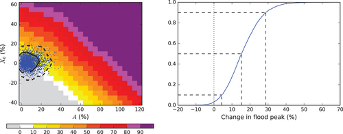
For each GMST change, the precipitation changes are overlaid on the flood response surfaces derived by Kay et al. (2021), for each 1 km river cell. The response surfaces for changes in 50-year return period flood peaks are applied here, with the extra uncertainty allowances (Section 2.1). For each 1 km river cell and each required GMST change, the impacts are extracted from the response surface and the cumulative distribution function (CDF) is plotted; changes in the flood peaks can be read from the CDF for any percentile of interest. This approach is illustrated in Figure 2.
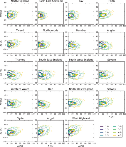
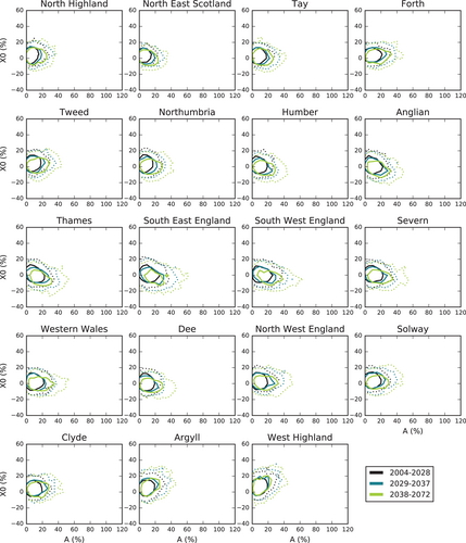
To test whether the incomplete ensembles for higher GMST changes are likely to lead to skewed flood peak changes, the precipitation changes for some of the lower GMST changes (with full ensembles) are split into three subsets by the time in the future at which the required GMST is reached. Contour plots comparing the subsets (Figure 4) show that ensemble members where the GMST change is reached later in the century tend to have some differences in the distribution of their corresponding precipitation changes, particularly in terms of greater seasonality (higher A), than those that reach the GMST change earlier. This dependence between the precipitation changes and the time in the future at which a certain GMST change is reached means that the flood peak changes extracted for incomplete ensembles (GMST changes of 3°C and above) will be skewed compared to those from complete ensembles (GMST changes of less than 3°C). Thus, a correction technique has been developed to account for this effect.
2.4 Correction for the effect of incomplete ensembles
To investigate the size of the effect of incomplete ensembles on the flood peak changes, the percentage of the ensemble members applied is systematically reduced (for GMST changes with full ensembles; 1.5, 2 and 2.5°C), to see how much difference this makes to the 50th percentile flood peak change compared to use of the whole ensemble. The percentage reductions in ensemble size applied are those corresponding to each of the required higher GMST changes (3, 3.5, 4 and 4.5°C; Table 1), and ensemble members are preferentially removed according to their corresponding time-slice and precipitation harmonic amplitude A (i.e., they are ordered first by time-slice, earlier to later, then by A, low to high, and ensemble members are systematically removed from the end of the ordered list). The differences derived for each percentage reduction in ensemble size for the lower GMST changes are then extrapolated, to estimate the difference for each of the required higher GMST changes. The ensemble corresponding to a 1°C GMST change is not used as part of the extrapolation, despite being a complete ensemble, as its strong concentration to the left-hand side of the sensitivity domain (Figure 3) regardless of time-slice, when combined with the response surfaces, introduces ‘noise’ into the extrapolation.
- Fit a straight line through the points for 1.5, 2 and 2.5°C.
- If the slope of the line is less than or equal to 0, extrapolate the line to the required GMST change (e.g., Figure 5a).
- If the slope of the line is greater than 0 (i.e., it would result in smaller estimates, and possibly positive values, for higher GMST changes), calculate the mean value of the points and use that to extrapolate instead (e.g., light green and orangey-yellow lines/dots in Figure 5b).
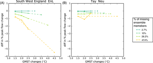
This process results in a table of estimated differences for each GB river-basin region, response type and required higher GMST change (3°C and above). The differences vary substantially by region and response type and generally increase with GMST change (see examples in Table 2), as would be expected with the increase in the percentage of the ensemble missing for higher GMST changes.
| Response type | South West England | Tay | ||||||
|---|---|---|---|---|---|---|---|---|
| 3°C | 3.5°C | 4°C | 4.5°C | 3°C | 3.5°C | 4°C | 4.5°C | |
| DpE | 0.0 | −0.1 | −0.8 | −1.5 | 0.0 | 0.1 | 0.0 | 0.5 |
| DpH | 0.0 | −0.3 | −1.1 | −1.5 | 0.0 | −0.1 | −0.2 | 0.2 |
| DpL | 0.0 | −0.2 | −1.3 | −3.5 | 0.0 | −0.4 | −0.4 | −0.3 |
| Neu | 0.0 | −0.3 | −1.7 | −4.4 | 0.0 | −0.3 | −0.4 | −0.7 |
| Mix | 0.0 | −0.3 | −1.2 | −2.4 | 0.0 | −0.2 | −0.4 | −0.2 |
| EnL | 0.0 | −0.5 | −1.9 | −5.5 | 0.0 | −0.1 | −0.4 | −0.7 |
| EnM | 0.0 | −0.4 | −1.9 | −5.1 | 0.0 | −0.3 | −0.2 | −0.5 |
| EnH | 0.0 | −1.0 | −3.1 | −6.7 | 0.0 | −0.5 | −0.4 | −0.7 |
| Sen | 0.0 | −0.5 | −2.4 | −4.7 | 0.0 | −0.4 | −0.2 | −0.2 |
- Abbreviations: GB, Great Britain; GMST, global mean surface temperature.
The representative flood response surfaces for each response type are used here, rather than the 1 km modelled response surfaces, to make the extrapolation fitting feasible; one for each response type, river-basin region, and percentage reduction in ensemble size (i.e., 9 × 19 × 4 = 684) rather than one for each 1 km river cell and percentage reduction in ensemble size (12,421 × 4 = 49,684).
3 RESULTS
3.1 Correction for the effect of incomplete ensembles
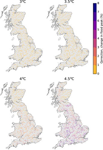
For each required higher GMST change (3°C and above), the table of differences in impact due to application of incomplete ensembles (Section 2.4) was used to assign a correction value to each 1 km river cell (using the river-basin region and response type of each river cell; Section 2.1.2). Any corrections below zero are set to zero, to avoid reducing the percentage change in flood peak. Figure 6 shows the resulting correction grids, illustrating the variable spatial pattern of corrections across Britain, and the larger adjustments required for percentage change estimates at 4.5°C. The appropriate correction grid is added to the 50th percentile flood peak change grid for GMST changes of 3°C and above.
3.2 Flood peak changes
Grids of 50th percentile changes in 50-year return period flood peaks were produced for each GMST change. As an example, Figure 7 maps the 50th percentile of change in 50-year return period flood peaks for 2 and 4°C GMST changes (including the correction for 4°C). They show significant spatial variation, with impacts typically higher in the west than the east. Additional grids of 10th and 90th percentile changes were produced for those GMST changes with (essentially) full 3000-member ensembles (1, 1.5, 2 and 2.5°C; Table 1), to illustrate the range of climate modelling uncertainty. Maps of the 10th and 90th percentile flood changes for a 2°C GMST change are included in Figure 7.
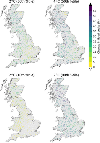
Figure 8 shows the regional means of the 50th percentile flood peak changes, both with and without the correction grids applied. This shows that the corrections make a relatively significant difference in some regions, especially for a 4.5°C GMST change (e.g., Tweed and South East England). Also shown in Figure 8 are the regional means of the 10th and 90th percentile flood peak changes for the lower GMST changes.
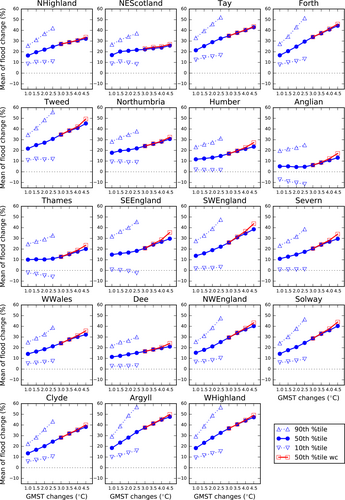
Anglian region has the lowest 50th percentile changes (~5% for 1–2.5°C) and the Tweed, Tay, Forth, Argyll and West Highland regions in Scotland have the highest changes (≥30% for GMST changes of 2.5°C). In contrast, the 10th percentile changes show decreases in flood peaks in some regions (e.g., Anglian and Thames). The 90th percentile changes can be significantly higher than the 50th percentile changes, especially for higher GMST changes. For example, the 50th percentile change for South East England for a 2.5°C GMST change is 18% but the 90th percentile change is 45%.
The regional means for the 50th percentile change for the four lower GMST changes (1–2.5°C) show increases in flood peaks with increasing GMST change, except for Thames (reasonably stable) and Anglian (slight decrease). Regions such as Forth and North West England show an approximately linear increase in flood peaks with increasing GMST change (~4%/0.5°C). Regions such as South West and South East England show accelerating flood peak changes with increasing GMST change. Thames region shows accelerating flood peak changes for GMST changes over 2.5°C.
4 DISCUSSION
4.1 Flood peak changes
The results presented here show the potential impacts of climate change on peak river flows across GB for a range of GMST changes (1–4.5°C). The study uses the latest probabilistic climate projections for the United Kingdom from UKCP18. Regional means for the 50th percentile change in 50-year return period flood peaks, for the four lower GMST changes (1–2.5°C), generally show increases in flood peaks. Such increases are consistent with previous studies using UKCP09 Regional climate projections (e.g., Bell et al., 2016; Collet et al., 2018; Kay & Jones, 2012), although none of these look at flood changes corresponding to specific GMST changes.
Regions such as South West and South East England would benefit the most from keeping GMST changes lower because their 50th percentile flood peak changes are estimated to accelerate with increases in GMST change. Some regions show decreases in the 10th percentile changes. This might be due to the reduction in summer seasonal mean rainfall which shows a strong north–south gradient, with greater reductions in rainfall in the south (figure 2.10 of Lowe et al., 2018). The 90th percentile changes can be significantly higher than the 50th percentile changes, especially for higher GMST changes, this may be due to much higher projected increases in winter seasonal mean precipitation (figure 2.9 of Lowe et al., 2018).
Several studies have estimated global and regional impacts at different temperature levels. Arnell et al. (2018) presented impact indicators (e.g., exposure to drought, river flooding and heat waves) using climate scenarios associated with specific GMST changes constructed by pattern scaling CMIP5 climate models, and investigated the impacts avoided if low temperature targets could be met. Others have used scenarios representing specific temperature targets constructed by ‘time-sampling’ (James et al., 2017) periods from a climate model simulation with the desired mean change in global temperature to estimate impacts on droughts (Naumann et al., 2018), extreme weather events and water availability (Schleussner et al., 2016), and crop yields (Ostberg et al., 2018). Arnell et al. (2021) demonstrate the sensitivity of climate risks in the United Kingdom to level of warming, and highlight the considerable regional variability in impact for some indicators, including flooding. This study used the response surfaces of Kay et al. (2021), onto which ‘time-sampled’ probabilistic projections were overlain to extract flood peak changes. This method has a number of advantages, including the ability to easily overlay large numbers of projections and the fact that new projections, that might be available at a later date, can be used to extract flood peak changes without having to re-run the hydrological model, that is, the response surfaces are independent of the climate model data (and its biases).
4.2 Sources of uncertainty
There are some limitations with this study, for example only one hydrological model is used which could underestimate the full uncertainty range in the results. Even though only one set of projections has been used, that set was designed to provide a wide representation of uncertainties. The UKCP18 Probabilistic projections were derived from a set of 360 climate model simulations including results from multi-model and perturbed parameter ensembles as well as accounting for uncertainties in physical processes and feedbacks at global and regional scales (Murphy et al., 2018).
Another source of uncertainty is the RCP trajectory, as a given GMST change can be obtained from simulations with different RCP trajectories. The effect of this was analysed (Supplementary Section 2.1), and the results show that the RCP trajectory used makes a difference to the impact estimates for a given GMST change; however, use of RCP8.5 emissions always gives the largest impacts of the four RCPs, and the differences are relatively small for the 50th percentile change.
The corrections for incomplete ensembles are done by response type, rather than for each 1 km cell separately, however the regional mean plots (Figure 8) suggest plausible patterns of change. The shape of the flood changes for higher GMSTs appears to follow the shape of the flood changes for lower GMSTs, rather than a change occurring at around a GMST change of 3°C (e.g., for SW England, with the correction the acceleration of flood changes with GMST changes seen for lower GMST changes continues for higher GMST changes, but without the correction the flood changes become approximately linear for higher GMST changes).
Other factors that could affect peak flow changes, such as potential future changes in land-cover/use, are not included in the estimation of peak flow changes.
4.3 Future flood risk
Extending the assessment of changes in peak flows to changes in flood risk is key to understanding the significance of potential changes and how they should be managed. This question is central to the five-yearly UK Climate Change Risk Assessment (CCRA), required under the Climate Change Act 2008, and in 2015 regional changes in peak flows where used within the Future Flood Explorer (FFE) to support CCRA2 (Sayers et al., 2015). The opportunity for a significantly improved spatial representation of changes in peak flows was taken forward in CCRA3, again using the FFE to provide insight into the associated changes in flood risk across a range of spatial reporting scales (Local Authorities up to UK-aggregated) given various scenarios of warming (2°C and 4°C rise in GMST), population growth and adaptation assumptions. Full details of the flood risk analysis process are provided by Sayers et al. (2020), but summarised here to illustrate the process.
The first step is to convert the change in peak flows into a change in river water levels by applying the Flood Estimation Handbook (FEH) statistical method (Kjeldsen et al., 2008) for the most appropriate 50 m FEH pixel for each G2G 1 km river cell. The FEH flood frequency curve for each grid point is used to estimate the change in the return period of the current T-year flood corresponding to a set of percentage changes in peak flow. In combination, this processing chain enables the FFE to capture the local context of the response to climate change and leads to highly spatially differentiated (credible) changes in extreme water levels, which is a significant advance over previous national-scale risk assessments. This highly spatially resolved approach recognises that two tributaries immediately upstream of a confluence can be quite different in their physical geography, meaning that nearby locations can have different flow responses; a variation not captured in regional-scale approaches to flood uplifts. How this change manifests in terms of a change in flood hazard will reflect the local defences (if present), the standard of protection that they afford and their condition (a consideration that adds further spatial differentiation). The change in flood hazard is then combined with information on exposure and vulnerability to assess the change in flood risk.
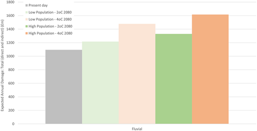
The results suggest that, at a UK-scale, fluvial flood risk is the dominant source of flood risk today (compared to coastal, groundwater and surface water) and remains so in the future (Sayers et al., 2020). The scale of future risk depends upon the combination of climate change, population growth and adaptation assumed to represent the future. Assuming a continuation of current levels of adaptation, Expected Annual Damage from fluvial flooding is projected to increase by the 2080s by about 9% given a 2°C rise in GMST and low population growth, and about 45% under a 4°C rise in GMST and high population growth (Figure 9).
5 CONCLUSIONS
Overlaying time-sampled sets of the UKCP18 Probabilistic projections on the flood response surfaces of Kay et al. (2021) has provided estimates of projected changes in 50-year return period flood peaks for 1 km river cells across GB corresponding to a range of GMST changes (from 1 to 4.5°C in 0.5°C increments). For GMST changes greater than 3°C, with incomplete ensembles, correction grids have been estimated.
By providing flood peak changes relative to levels of GMST change, rather than by future time-slice and emission scenario as done previously, the results directly illustrate the additional impact that higher levels of GMST change could have, regardless of the future time-period in which the level is reached or what emissions trajectory is followed. This helps to address the increasing demand from policymakers for evidence on the potential impacts of specific levels of change in GMST (Arnell et al., 2019, 2021). Other studies have presented large-scale global and regional impacts of climate change on floods for specific GMST changes, but this study goes further by providing 1 km-scale impact projections for GB.
The results of this study have also fed into the most recent five-yearly UK CCRA (Defra, 2012; Defra, 2017; Defra, 2022), where they have been used within the FFE to underpin the translation of changes in flood peaks into changes in fluvial flood risk given alternative adaptation assumptions (Sayers et al., 2020). This translation to flood risk is key to understanding the significance of the potential changes and how they should be managed.
ACKNOWLEDGEMENTS
This research was funded by The Climate Change Committee (CCC) and forms part of the Third Climate Change Risk Assessment (CCRA3) Floods report (Sayers et al., 2020).
Open Research
DATA AVAILABILITY STATEMENT
The UKCP18 data are available from CEDA. The regional results from the Future Flood Explorer (FFE) CCRA3 analysis are available at https://www.ukclimaterisk.org/wp-content/uploads/2020/09/CCRA3-Results-Summary-External-02Sept2020.xlsx. Other data are available from the authors upon reasonable request.


