1 INTRODUCTION

Melting of snow and glaciers at high altitude mountains are important sources of freshwater (Barnett et al., 2005; Kaser et al., 2010). Climate change is varying glacier runoff by increasing summer ablation of glaciers and decreasing winter accumulation throughout the world (Pellicciotti et al., 2010). The Hindukush ranges and Himalaya–Karakoram (HK) region are characterized by a higher degree of complexity and variability in snow accumulation, snow and glacier melt than the overall response of glacierized basins (Hewitt, 2005) in many countries of central Asia and South Asia, namely, China, Pakistan, India, Nepal, Afghanistan, and so forth. Many broader aspect studies have been conducted on these mountain regions (Immerzeel et al., 2012; Singh et al., 2006; Singh & Bengtsson, 2004; Singh & Jain, 2002; Singh & Kumar, 1997). However, the particular response of climate change is also necessary to be examined as a case study regarding Pakistan's water resources which can further be applied in similar mountainous source regions.

Pakistan is mainly an agrarian economy that depends heavily on its irrigation water supplies from the Indus River and its tributaries. More than 30% of the hydropower and approximately 95% of the irrigation water demand of Pakistan are fulfilled by the Indus Basin irrigation system (Pritchard, 2017). Thus, major agricultural areas of Pakistan (e.g., Punjab and Sindh provinces) depend on the irrigation water supplies from the source region of the Indus River (SRIR), consisting of the upper Indus River basin (UIRB), Kabul River basin (KRB), and Jhelum River basin (JRB) (Rizwan et al., 2019). SRIR also possesses large groundwater resources in its alluvial aquifers. However, groundwater resources are under severe threat due to poor recharge and anthropogenic pollution including the agriculture sector (Hamid & Lee, 2016). The Indus River originates from Lake Manasarovar on the Tibetan Plateau (TP) and flows through the Himalayas, Karakoram, and Hindukush (HKH) ranges to the Arabian Sea. Yao et al. (2012) reported that high mountainous and large cryospheric areas of the HKH region have a significant impact on the atmospheric circulation systems of world and particularly of Asia. The main river basins of the SRIR in the HKH region have different atmospheric circulation systems (Ali et al., 2019). The main part of the UIRB lies in the Karakoram ranges and experiences westerlies and monsoon circulation systems (Tahir et al., 2016). The southeastern part of this basin is in the TP and experiences the southeastern monsoon circulation system (Dahri et al., 2016). The JRB is in the Himalayan ranges and experiences the monsoon circulation system of the Arabian Sea, Indian Sea, and Bay of Bengal (Tahir et al., 2016). Water from the JRB is stored in Mangla Dam which is the second largest dam and one of the largest hydropower generators in Pakistan. Mangla dam has a storage capacity of about 7.4 MAF and is a major source of irrigation water for Indus Basin. The KRB is in the Hindukush ranges and experiences westerly disturbances from the Mediterranean Sea and Caspian Sea (Filippi et al., 2014). Pakistan receives water from KRB and stores it in Warsak Dam, constructed on the Kabul River which is another source of hydropower generation and irrigation in Khyber Pakhtunkhwa province.

A change in atmospheric temperature and precipitation (especially in snow-dominated watersheds) affects the flow in the rivers (Deng et al., 2015; Lutz et al., 2014). It has been reported that seasonal water supplies are affected by changes in temperature, while runoff volumes are affected by changes in precipitation and snow accumulation (Anjum et al., 2018; Sharma et al., 2016). Rizwan et al. (2019) reported that precipitation in the SRIR has an increasing trend, that is, 19 mm/decade in the UIRB, 34 mm/decade in the KRB, and 36.6 mm/decade in the JRB. It has also been reported that the temperature is increasing in the upper Indus basin (Azmat et al., 2017; Tahir et al., 2016). Long-lasting variations in temperature and precipitation have diverse effects on the hydrological regimes of the UIRB (Mahmood & Jia, 2016). An increasing trend of heavy precipitation and a decreasing trend of number of rainy days in the SRIR will result in significantly enhanced risks of flash flood events (Rizwan et al., 2019). It is also feared that a persistent change in climatic conditions may further aggravate this scenario.

Flooding is one of the most destructive and complicated environmental disasters in Pakistan and occurs due to (1) natural factors, that is, extreme precipitation in the Indus River and its tributaries during the monsoon season (Khalid et al., 2013), and (2) anthropogenic factors, that is, settlements in flood plains, lack of water reservoirs to absorb flood peaks and inappropriate flood prediction and control systems (Federal Floods Commission, 2016). During 2010, Pakistan suffered from one of the largest flood disasters in its history as it affected approximately 20% of the country's total land area, 20 million people and caused economic losses in the billions (Webster et al., 2011). It is, therefore, compelling to address anthropogenic factors. The development of new infrastructure is a long and expensive process that requires accurate predictions of future needs as well as information on the magnitudes of extreme flows and flood events. In addition, the development of early flood warning and prediction systems using simulation tools can help cope with floods and minimize expected damage even in the presence of sufficient structural measures (Aziz & Tanaka, 2011). The forecasting of the future water availability (especially in changing climate scenarios) is also very important for Pakistan, as its agriculture mainly depends on fresh water from the SRIR (Mahmood & Jia, 2016; Tahir et al., 2016).

To evaluate the climate change effects on different river basins hydrological responses, the results of different climate models were used as input (Basheer et al., 2016; Garee et al., 2017). According to Almazroui et al. (2017) and Singh and Goyal (2016), the global atmosphere can be represented well using CMIP5-based climate model outputs. According to a study conducted by Babur et al. (2016) in the Himalayan ranges, changes in the annual average temperature and precipitation are projected, that is, up to 4.65°C and 43% under RCP4.5 and 7.81°C and 51% under RCP8.5, respectively, in the 2080s time horizon. Most of the previous studies on future projection focused on the HK ranges under the RCP4.5 and RCP8.5 scenarios. For example, it has been reported that river flows at the end of this century are expected to increase by 10% in the Karakoram ranges (Garee et al., 2017) and 15% in the Himalayan ranges (Mahmood & Jia, 2016). However, studies in the Hindukush ranges are limited and no study has been conducted in the whole SRIR under RCP2.6, RCP4.5, and RCP8.5 for investigations of future floods and water availability. This study focused on the investigation of historical and future floods in the SRIR using an integrated flood analysis system (IFAS) model because of its capability of simulating floods at any point in the basin. Miyamoto et al. (2014) modeled the Cagayan River basin in Philippines for effective flood prediction. They used satellite and ground rainfall in IFAS model for flood prediction and found very good results. Hafiz et al. (2013) successfully modeled Dungun River basin in Malaysia for prediction of floods, with coefficient of efficiency computed as 0.72 using IFAS model. The main objective of conducting this research study was to simulate the projected daily stream flows of the main rivers of the SRIR (i.e., Indus, Kabul, and Jhelum) using the IFAS for the investigation of future floods in near future (2020–2059) and far future (2060–2099) periods. The model was calibrated for historical stream flow data for the years 1976–1995 and validated for the years 1996–2015.

2 STUDY AREA AND DATASETS

2.1 Study area

This study was conducted in the SRIR (Figure 1), which provides fresh water to all sectors of the Pakistani economy. The study area is the upper part of the transboundary Indus basin shared by Pakistan, India, and Afghanistan. It consists of three main river basins, of which the upper Indus is the largest river basin and Jhelum is the smallest river basin. The summer season is short and mild, while the winter season is harsh and long in the study area. The UIRB consists of mountainous areas of uneven terrain, while the KRB and JRB consist of comparatively smooth areas. The JRB receives the highest amount (1014 mm) of annual precipitation, while the UIRB receives the minimum amount (226 mm) of annual precipitation.

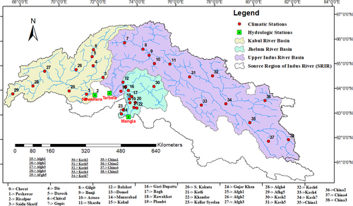
The largest portion of stream flow is contributed by precipitation in the JRB and by glacier and snow melt in the KRB and UIRB (Dahri et al., 2016). According to the observed stream flow data from 1976 to 2015, the average annual discharge from the UIRB at Tarbela, the KRB at Nowshera, and the JRB at Mangla was 2439, 818, and 819 m³/s, respectively.

2.2 Datasets

Table 1 shows the main datasets which were used for the investigation of historical and projected flood events in the study area.

TABLE 1. Datasets used in the study.

Data category	Dataset	Period	Data source
Hydrology	Stream flow	1976–2015	Water and Power Development Authority (WAPDA)
Climate (observed)	Air temperature and precipitation	1976–2015	Water and Power Development Authority (WAPDA) and Pakistan Meteorological Department (PMD)
Climate (gridded)	Air temperature and precipitation	1976–2015	APHRODITE
Soil	Digital map of soil and its properties		FAO and UNESCO
Land cover	Data of land use		International Steering Committee for Global Mapping (ISCGM)
Future climate	Projected data of air temperature and precipitation	2020–2099	NASA Earth Exchange Global Daily Downscaled Projections (NEX-GDDP)

• Abbreviations: FAO, Food and Agriculture Organization; UNESCO, United Nations Education, Scientific, and Cultural Organization.

2.2.1 Climate data-observed

Daily recorded precipitation, maximum and minimum temperature during the period of 1976–2015 of 24 climatic stations located within the premises of Pakistan were obtained from the Water and Power Development Authority (WAPDA) and Pakistan Meteorological Department and the same data for the same time period of 14 climatic stations located outside the boundary of Pakistan was extracted from APHRODITE, while the daily stream flow data were also obtained from the WAPDA.

APHRODITE is developed by an association between the Research Institute for Humanity and Nature Japan and the Meteorological Research Institute of the Japan Meteorological Agency. APHRODITE precipitation data have also been used by Tahir et al. (2011) along with the snowmelt runoff model in one sub-basin of the SRIR.

2.2.2 Climate data-based on general circulation models

The projected precipitation, maximum and minimum temperature data from six climate models were downloaded from the Model for Interdisciplinary Research on Climate Version 5 (CMIP5) data archive for low (2.6 W/m²), medium (4.5 W/m²), and high (8.5 W/m²) radiative forcing scenarios (i.e., RCP2.6, RCP4.5, and RCP8.5, respectively). The general circulation model (GCM)-based future data on precipitation and maximum and minimum temperatures under RCPs for the period of 1976–2099 were downloaded and divided into three groups, that is, baseline period (1976–2015), near future period (2020–2059), and far future period (2060–2099). The features of selected GCMs are presented in Table 2. To carry out the analysis on equivalent resolutions at the basin scale, the delta downscaling and bias correction method was used to downscale and bias correct the projected data of GCMs.

TABLE 2. Features of six general circulation models (GCMs) under RCP2.6, RCP4.5, and RCP8.5.

GCM	Research center	Location	Time scale	Resolution
bcc-csm1-1	Beijing Climate Center	China	Daily	0.25° × 0.25°
BNU-ESM	Beijing Normal University	China	Daily	0.25° × 0.25°
MPI-ESM-LR	Max Planck Institute	Germany	Daily	0.25° × 0.25°
IPSL-CM5A-LR	Institut Pierre-Simon Laplace	France	Daily	0.25° × 0.25°
IPSL-CM5A-MR	Institut Pierre-Simon Laplace	France	Daily	0.25° × 0.25°
GFDL-ESM2M	Geophysical Fluid Dynamics Laboratory	USA	Daily	0.25° × 0.25°

• Abbreviation: GCM, general circulation model.

2.2.3 Land cover data

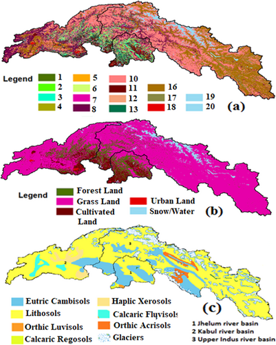
Considering the importance of land cover for the generation of stream flow in the study area, we used global map land cover data (1 km × 1 km spatial resolution) provided by the International Steering Committee for Global Mapping. Nineteen classes of land cover were identified in the study area (Figure 2a). A description of each class of land cover is given in Table 3. Land cover data was used to estimate the parameters of the surface tank in the IFAS model. According to Sugiura et al. (2014), the land cover classes were mainly grouped into urban land, forestland, cultivated land, grassland and water, and snow because of the large number of parameters of the surface tank. The final five classes of land cover distribution are presented in Figure 2b.

TABLE 3. Global land cover and IFAS surface tank parameter class (Sugiura et al., 2014).

Sr. no.	Global map categories	IFAS parameter
1	Broadleaf evergreen forest	1
2	Broadleaf deciduous forest
3	Needle leaf evergreen forest
4	Needle leaf deciduous forest
5	Mixed forest
6	Tree open
7	Shrub	2
8	Herbaceous
9	Herbaceous with sparse tree/shrub
10	Sparse vegetation
11	Bare area consolidated (gravel, rock)
12	Bare area unconsolidated (sand)
13	Cropland	3
14	Paddy field
15	Cropland/other vegetation mosaic
16	Mangrove
17	Wetland
18	Urban	4
19	Snow/ice	5
20	Water bodies

• Abbreviation: IFAS, integrated flood analysis system.

2.2.4 Soil data

Soil data of the study area was obtained from the Digital Soil Map of the World developed by the Food and Agriculture Organization and United Nations Education, Scientific, and Cultural Organization. The soil data was used directly in the IFAS model to estimate the parameters of the aquifer tank. The distribution of soil classes in the study area is shown in Figure 2c.

3 METHODOLOGY

4 RESULTS

4.1 Future changes in precipitation and temperature

In this study, the performance of the selected GCMs is assessed by the Taylor diagram approach and results are presented in Figure 3. Taylor diagrams are capable of providing performance insight through comparison of GCMs and baseline periods data sets with reference to standard deviation (SD), CC and root mean square error (RMSE). The black dotted lines and gray lines denote the values of CC and RMSE, respectively, while the values of x-axis and y-axis represent SD. The downscaled climatic variables, that is, precipitation, maximum, and minimum temperature from all the selected GCMs especially their ensemble showed good agreements with the gauge based data set of the base line period, as witnessed by low SD and RMSE values and high CC values.

Average changes in projected precipitation and maximum and minimum temperatures (mean areal of the study area) in the near future period (2020–2059) and far future period (2060–2099) relative to the historical period (1976–2015) under the RCP2.6, RCP4.5, and RCP8.5 scenarios are shown in Table 4.

TABLE 4. Average changes (%) in SRIR during future time horizons relative to baseline period.

Climate models	Time period	Precipitation			Maximum temperature			Minimum temperature
		RCP2.6	RCP4.5	RCP8.5	RCP2.6	RCP4.5	RCP8.5	RCP2.6	RCP4.5	RCP8.5
bcc-csm1-1	2020–2059	140	94	77	3.3	3.6	3.8	0.0	0.2	0.7
	2060–2099	102	147	191	3.0	4.2	6.6	0.0	0.8	2.7
BNU-ESM	2020–2059	192	221	163	3.9	3.6	4.1	0.2	0.1	1.6
	2060–2099	249	174	228	4.1	5.2	7.4	0.9	2.1	4.7
GFDL-ESM2m	2020–2059	130	85	125	2.0	2.6	3.6	1.2	1.3	1.9
	2060–2099	52	95	117	1.7	3.2	6.1	0.5	2.2	3.6
IPSL-CM5A-LR	2020–2059	78	-8	63	2.6	3.8	8.4	1.5	1.5	4.1
	2060–2099	108	64	44	2.9	5.5	11.9	1.2	2.3	7.3
IPSL-CM5A-MR	2020–2059	89	35	84	3.1	4.1	4.6	1.5	1.8	1.7
	2060–2099	60	139	209	3.3	6.1	8.4	1.2	2.9	5.2
MPI-ESM-LR	2020–2059	33	44	90	2.8	3.3	3.8	2.2	1.7	1.2
	2060–2099	100	57	127	1.3	4.3	7.3	−0.5	1.5	3.6
ensemble	2020–2059	111	79	100	0.5	0.8	2.1	3.9	4.3	4.9
	2060–2099	112	113	153	0.7	2.0	5.3	3.8	5.1	7.4

• Abbreviation: SRIR, source region of the Indus River.

The projected precipitation of all climate models showed positive changes in both future periods under the RCP scenarios except for one climate model, which showed a negative change in the near future period under RCP4.5. Annual average changes in projected precipitation higher than 100% were observed in many climate models in the near future period and far future period. Positive probable changes in annual maximum temperature were observed in all climate models, with 0.5–4.1°C under RCP2.6, 0.8–6.1°C under RCP4.5, and 2.1–11.9°C under RCP8.5. One climate model showed a negative change in annual minimum temperature, while all other climate models showed positive changes. During both periods (near future and far future), −0.5–3.9°C, 0.1–5.1°C, and 0.7–7.4°C changes are expected in annual minimum temperature under RCP2.6, RCP4.5, and RCP8.5, respectively. As expected, higher changes were observed under RCP8.5, and lower changes were observed under RCP2.6.

4.2 Calibration and validation of the IFAS model

Different parameters, such as the surface and subsurface tank model, aquifer tank model and river course tank model, were calibrated to suit the physical characteristics of the study area. Selected parameters for calibration of IFAS model are shown in Table 5. Finally, the calibrated parameters were tested against the daily recorded stream flows during the validation period. To warm up, the IFAS model was run at least 6 months earlier than a flood event to obtain the preflood base conditions, which were then used for the simulation of a main flood event. Daily observed data from 1976 to 1995 were used for calibration, while data from 1996 to 2015 were used for validation of the simulated results. Figure 4 exhibits the comparison between observed versus simulated stream flows.

TABLE 5. Parameters used in the IFAS model.

Surface parameters
S. No.	fo (infiltration capacity)	Sf2 (maximum storage height)	Sf1 (rapid intermediate flow)	Sfo (height where ground infiltration occurs)	N (surface roughness coefficient)	αn (rapid intermediate flow regulation coefficient)	Initial storage height (m)
1	0.00001	0.06	0.01	0.002	1	0.15	0
2	0.00002	0.08	0.01	0.002	3	0.2	0
3	0.00001	0.09	0.01	0.005	3.5	0.3	0
4	0.000001	0.05	0.0005	0.0001	2.1	0.25	0
5	0.000001	0.09	0.01	0.005	4.5	0.3	0

Aquifer parameters
AUD (1/mm/day)1/2	AGD (1/day)	HCGD (m)	HIGD (m)
0.2	0.0003	2	2
0.21	0.0003	2	2
0.22	0.0003	2	2
0.23	0.0003	2	2

River course parameters
S. No.	RBW	RBS	RNS	RRID	RGWD	RHW	RHS	RBH	RBET	RLCOF
1	7	0.5	0.038	0.2	0	9999	1	0.5	0.05	1.4
2	7	0.5	0.037	0.2	0	9999	1	0.5	0.05	1.4
3	7	0.5	0.036	0.2	0	9999	1	0.5	0.05	1.4

• Note: Explanation of aquifer and river course parameters is as follows: AUD, unconfined aquifer runoff coefficient; ADG, confined aquifer runoff coefficient; HCGD, storage height for unconfined aquifer; HIGD, initial value for calculation; RBW, coefficient for actual river width; RBS, coefficient approximately to 0.3–0.5; RNS, Manning coefficient; RRID, initial value for calculation; RGWD, infiltration coefficient from river to aquifer layer tank; RHW, water level of submerged high water channel; RHS, water level of submerged low water channel; RBH, river width of high water channel/low water channel; RBET, slope gradient of high water channel; RLCOF, collection coefficient of river length.

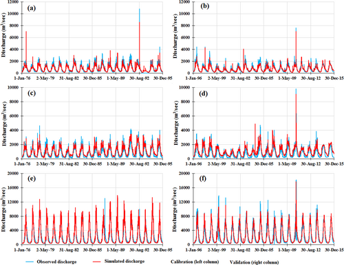
The model successfully simulated the flood event that occurred during 2010 in all three river basins of the study area. IFAS model was evaluated by comparing the observed and simulated stream flows, and good correlation is observed in all three river basins, with R² = 0.90 and 0.89 (Mangla), 0.89 and 0.86 (Nowshera), and 0.92 and 0.93 (Tarbela) during calibration and validation, respectively (Figure 5).

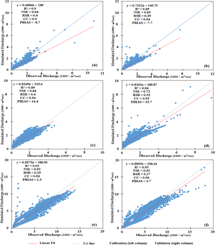
The NSE values in the JRB, KRB, and UIRB were higher than 0.5, showing that the simulated results were acceptable. Similarly, the values of RSR, CC, and PBIAS in the main river basins of the study area during both periods (calibration and validation) were within their acceptable ranges, which means that the model could simulate the stream flows efficiently under the projected climate conditions. The calculated values of these statics in the UIRB showed higher accuracy than those in the other two river basins of the study area.

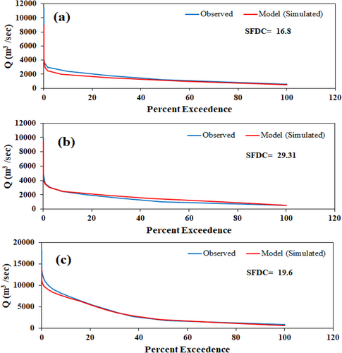
Figure 6 shows the flow duration curves for the validation of the IFAS simulated stream flows for the main river basins of the study area. Calculated values of SFDC for JRB, KRB, and UIRBs are 16.8, 29.31, and 19.6, which are within the acceptable ranges.

4.3 Projected stream flows under climate change scenarios

4.3.1 Annual average changes

The annual average stream flow during the baseline period of the JRB, KRB, and UIRB was used to calculate the projected stream flow anomalies, and the results are presented in Figures 7-9 for JRB, KRB, and UIRB, respectively. An increase in the projected stream flow is shown by a positive anomaly, while a negative anomaly represents a decrease in the projected stream flow. In the JRB, four climate models, that is, bcc-csm1-1, BNU-ESM, GFDL-ESM2M, and IPSL-CM5A-LR showed positive and negative changes in projected flows ranging between −100% and 150%, two climate models, that is, IPSL-CM5A-MR and MPI-ESM-LR showed changes between −100% and 100%, and mostly negative anomalies were observed in the ensemble of these climate models (Figure 7). In the KRB, mostly positive anomalies were observed, ranging from −50% to 500% in the six climate models and −50% to 150% in the ensemble (Figure 8). Higher values of anomalies were noted under RCP2.6 and RCP4.5, while lower values were observed under RCP8.5 in the ensemble. Positive anomalies in the UIRB, ranging from −10% to 250% in the climate models and 0 to 150% in the ensemble, showed an increase in the projected stream flow. The projected stream flow increased gradually under RCP8.5 and RCP4.5, while the same model predicted a slight decrease under RCP2.6 in the projected time period (Figure 9).

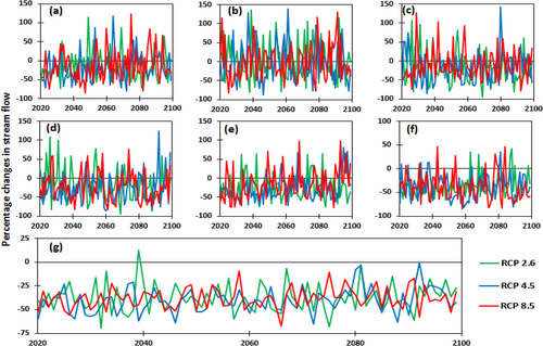
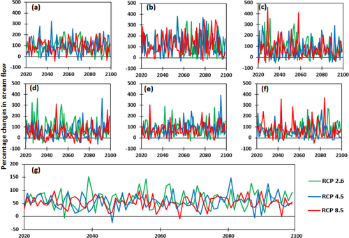
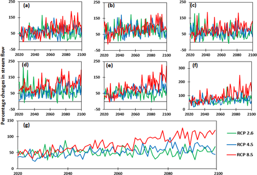
The annual average changes in the projected stream flows is determined by comparing it with that of the historical/baseline period of the JRB, KRB, and UIRB and results are presented in Table 6. The projected stream flow investigation in the JRB predicted that the annual average stream flow in the near and far future time periods could decrease at a rate of −4% to −43% in all climate models except in one model, that is, BNU-ESM, which showed a slight increase in stream flow under the RCP scenarios. All climate models during both future time horizons showed increases in the annual average stream flows under RCP2.6, RCP4.5, and RCP8.5 in the KRB and UIRB at rates of 47%–138% and 46%–124%, respectively. An analysis of projected stream flows showed that annual average flow in the ensemble of climate models could decrease at a rate of −37% to −43% in the JRB, while it is expected to increase at a rate of 53%–67% in the KRB and 47%–95% in the UIRB under the RCP scenarios. Munawar et al. (2021) and Anjum et al. (2019) also confirm the decrease and increase in the simulated average annual flows in their studies on JRB and Swat River basin (part of Kabul basin), respectively. According to Mahmood and Jia (2016), the simulated stream flow showed a reduction in the summer season in JRB.

TABLE 6. Average changes (%) in projected stream flow in the future time horizons.

Climate models	Time period	Jhelum River basin			Kabul River basin			Upper Indus River basin
		RCP2.6	RCP4.5	RCP8.5	RCP2.6	RCP4.5	RCP8.5	RCP2.6	RCP4.5	RCP8.5
bcc-csm1-1	2020–2059	−16	−25	−24	101	88	83	59	60	54
	2060–2099	−20	−9	−5	86	93	104	57	70	97
BNU-ESM	2020–2059	5	2	−5	122	120	109	74	75	71
	2060–2099	5	−4	3	138	119	133	80	80	99
GFDL-ESM2m	2020–2059	−8	−22	−9	103	82	89	66	60	71
	2060–2099	−24	−16	−13	67	75	60	53	66	90
IPSL-CM5A-LR	2020–2059	−9	−31	−17	102	52	50	72	46	87
	2060–2099	−24	−22	−28	67	71	47	58	73	113
IPSL-CM5A-MR	2020–2059	−25	−33	−24	91	68	69	52	48	60
	2060–2099	−25	−17	−9	84	102	83	50	79	116
MPI-ESM-LR	2020–2059	−43	−38	−35	63	60	86	59	60	71
	2060–2099	−30	−37	−41	106	58	70	74	73	124
ensemble	2020–2059	−38	−43	−39	64	54	54	51	47	60
	2060–2099	−37	−37	−37	67	58	53	52	62	95

This is because the major portion of the stream flows in these two basins (KRB and UIRB) comes from the melting of snow/glacier which increases with the increase of temperature while in JRB, the stream flow is mainly comprised of rainfall. A possible explanation for the reduction in stream flows perhaps is the decrease in the monsoon rainfall in the study area.

4.3.2 Temporal changes in mean monthly stream flow

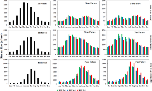
A comparison of temporal changes in the mean monthly stream flow of ensembles of climate models versus the historical period was considered in the study area, and the results are presented in Figure 10. Every year from May to July, a high flow rate was observed in the study area. Based on historical data, the highest flow was recorded during May–June in the JRB, which is expected to shift to April–May and August–September in the near and far future time horizons, respectively. This shift is perhaps linked with westerlies circulation and shifting of the monsoon because of climate change. In the UIRB, the highest flow months are the same in the future periods as in the historical period (July–August), while they are expected to shift from June–July (historical) to April–May (future) in the KRB. Overall, a decrease of 54%–60% is estimated in the projected stream flow in the JRB, while increases of 5%–12.5% and 24%–50% are projected in the mean monthly stream flow of the highest flow months of the KRB and UIRB under the RCP scenarios, respectively.

4.3.3 Number of flood events

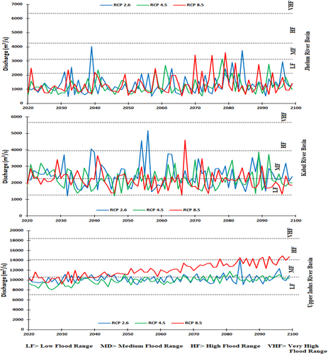
The temporal distribution of simulated flood events of different categories such as low floods, medium floods, high floods, and very high floods based on the flood limits of these rivers (Table 7) are presented in Figure 11. The number of flood events in the main river basins of the study area under RCP2.6, RCP4.5, and RCP8.5 during 2020–2059 and 2060–2099 was assessed and the results are presented in Table 8.

TABLE 7. Flood limits of main rivers of the study area.

Flood categories	Jhelum River basin at Mangla	Kabul River basin at Nowshera	Upper Indus River basin at Tarbela
	Discharge in m3/s
Low flood	2124–3114.9	1274–2264.9	7079–10618.9
Medium flood	3115–4247.9	2265–3963.9	10,619–14157.9
High flood	4248–6370.9	3964–5662.9	14,158–18405.9
Very high flood	≥6371	≥5663	≥18,406

• Source: Pakistan Meteorological Department, Flood Forecasting Division.

TABLE 8. Number of events of different categories of floods.

Climate models	RCPs	Time period	Jhelum River basin				Kabul River basin				Upper Indus River basin
			LF	MF	HF	VHF	LF	MF	HF	VHF	LF	MF	HF	VHF
Ensemble of GCMs	2.6	2020–59	2	1	0	0	16	20	3	0	29	11	0	0
		2060–99	4	1	0	0	17	23	0	0	25	15	0	0
	4.5	2020–59	2	0	0	0	21	18	0	0	39	1	0	0
		2060–99	4	1	0	0	25	15	0	0	26	14	0	0
	8.5	2020–59	4	0	0	0	19	21	0	0	16	24	0	0
		2060–99	4	3	0	0	26	12	1	0	0	30	10	0

• Abbreviations: GCM, general circulation model; HF, high flood; LF, low flood; MF, medium flood; VHF, very high flood.

As climate models have uncertainties in their climate data, these uncertainties are minimized by using an ensemble of these models. High flood events are expected in the KRB and UIRB. The JRB is expected to have the least number of low to medium flood events, while the KRB and UIRB are expected to have a large number of low to medium flood events. Ten events of high floods are expected in the UIRB during 2060–2099 under RCP8.5, and no high flood event is expected under RCP2.6 and RCP4.5 in the study area.

5 DISCUSSION

The study area, that is, SRIR, situated on the HKH ranges and in the TP region, provides fresh water for irrigated agriculture in the Indus Basin, and is very sensitive to climate change (Anjum et al., 2018; Rizwan et al., 2019). Climate change impact on stream flows can be assessed using the (GCMs outputs) (Jiang et al., 2015; Su et al., 2016). The goal of this study was to assess the probable impacts of climate change on floods in the SRIR using an IFAS model. For that purpose, the outputs of six GCMs under RCP2.6, RCP4.5, and RCP8.5 were downscaled and divided into two time horizons, that is, near future period (2020–2059) and far future period (2060–2099). Climatic parameters downscaled from six GCMs used in this study are in good agreement with the recorded observations (gauge based) during the historical period (1976–2015). CMIP5-based climate models have comparatively higher ability to reproduce the climatic parameters in the study area (Babur et al., 2016; Garee et al., 2017). The analysis of six GCMs and their ensemble's output used in this study showed increase in annual average precipitation during both future periods. A study conducted by Zhang et al. (2015) also showed similar results in the headwaters of Yellow River basin. A persistently increasing trend in annual precipitation is reported by Babur et al. (2016) and Garee et al. (2017) in their respective studies conducted in HK range, respectively. The possible reason for this increase might be linked with the westerlies circulation system, that is, a dominant circulation system in the Hindukush ranges (Anjum et al., 2018). Also, higher amounts of anthropogenic absorbing aerosols in the South Asian atmosphere may the reason for the increase in annual precipitation (Kaskaoutis et al., 2018). All six GCMs used in this study showed continuous increase in the annual temperature that is also reported by different researchers in their studies conducted in nearby South Asian regions (Dimri et al., 2018; You & Kang, 2016). Yan et al. (2016) and Anjum et al. (2018) reported that higher amounts of aerosols and greenhouses gasses might be the possible reason for this significant increase in the temperature.

The simulated results of stream flow from IFAS hydrologic model showed an increase in KRB and UIRB. Similar results are also reported by Immerzeel et al. (2013). The simulated results showed a decrease in the JRB. A possible reason for the increase in projected stream flows of the Kabul and upper Indus basins is that more than 70% of stream flows comes from snow/glacier melts thus increasing temperature will result in higher melting rates and ultimately the flow will also increase. Moreover, the time of occurrence of projected peak flows is expected to move to April–May in Jhelum and Kabul basins that might be linked with winter precipitation (westerlies circulation system) in the Himalayan and Hindukush ranges.

The foremost limitation of this research work is not considering the effects of climate change on the vegetation. Zhang et al. (2011) reported that changes in vegetation have significant effects on the stream flow. Another limitation is that the model used in this study lacks snowmelt and glacier melt functions. However, snow and glacier melt is calculated by a degree day method along with air temperature and fractional snow/glacier cover for discharge simulation. Future research should be carried out using hydrologic models which support snow and glacier melts and its results need to be compared with the results of this study.

6 UNCERTAINTIES

The foremost uncertainty is associated with the unavailability of adequate gauge based climatic data in the study area. Insufficiency of climatic data was managed by using APHRODITE precipitation for those stations which are outside the boundary of Pakistan. APHRODITE precipitation is claimed to be underestimated at higher mountains which needs to be adjusted (Immerzeel et al., 2015; Wortmann et al., 2018).

7 CONCLUSION

This study concentrated on future changes in temperature and precipitation and ultimately their influences on stream flows of the study area. The results revealed that the projected stream flow in the study area will increase with multiple flood events. Snow and glacier melting is also expected to accelerate with increasing temperature under RCP8.5 in the UIRB, which may cause flash floods. Therefore, it is very important to make management plans to cope with floods, save infrastructure and human lives and reduce flood damage.