Volume 16, Issue 1 e12854

ORIGINAL ARTICLE

Open Access

Exploring the role of the long short-term memory model in improving multi-step ahead reservoir inflow forecasting

Xinran Luo,

Xinran Luo

State Key Laboratory of Water Resources and Hydropower Engineering Science, Wuhan University, Wuhan, China

Hubei Provincial Key Lab of Water System Science for Sponge City Construction, Wuhan University, Wuhan, China

Search for more papers by this author

Pan Liu,

Corresponding Author

Pan Liu

[email protected]

orcid.org/0000-0002-3777-6561

State Key Laboratory of Water Resources and Hydropower Engineering Science, Wuhan University, Wuhan, China

Hubei Provincial Key Lab of Water System Science for Sponge City Construction, Wuhan University, Wuhan, China

Correspondence

Pan Liu, State Key Laboratory of Water Resources and Hydropower Engineering Science, Wuhan University, Wuhan 430072, China.

Email: [email protected]

Search for more papers by this author

Qianjin Dong,

Qianjin Dong

State Key Laboratory of Water Resources and Hydropower Engineering Science, Wuhan University, Wuhan, China

Hubei Provincial Key Lab of Water System Science for Sponge City Construction, Wuhan University, Wuhan, China

Search for more papers by this author

Yanjun Zhang,

Yanjun Zhang

State Key Laboratory of Water Resources and Hydropower Engineering Science, Wuhan University, Wuhan, China

Hubei Provincial Key Lab of Water System Science for Sponge City Construction, Wuhan University, Wuhan, China

Search for more papers by this author

Kang Xie,

Kang Xie

State Key Laboratory of Water Resources and Hydropower Engineering Science, Wuhan University, Wuhan, China

Hubei Provincial Key Lab of Water System Science for Sponge City Construction, Wuhan University, Wuhan, China

Search for more papers by this author

Dongyang Han,

Dongyang Han

State Key Laboratory of Water Resources and Hydropower Engineering Science, Wuhan University, Wuhan, China

Hubei Provincial Key Lab of Water System Science for Sponge City Construction, Wuhan University, Wuhan, China

Search for more papers by this author

Xinran Luo,

Xinran Luo

State Key Laboratory of Water Resources and Hydropower Engineering Science, Wuhan University, Wuhan, China

Hubei Provincial Key Lab of Water System Science for Sponge City Construction, Wuhan University, Wuhan, China

Search for more papers by this author

Pan Liu,

Corresponding Author

Pan Liu

[email protected]

orcid.org/0000-0002-3777-6561

State Key Laboratory of Water Resources and Hydropower Engineering Science, Wuhan University, Wuhan, China

Hubei Provincial Key Lab of Water System Science for Sponge City Construction, Wuhan University, Wuhan, China

Correspondence

Pan Liu, State Key Laboratory of Water Resources and Hydropower Engineering Science, Wuhan University, Wuhan 430072, China.

Email: [email protected]

Search for more papers by this author

Qianjin Dong,

Qianjin Dong

State Key Laboratory of Water Resources and Hydropower Engineering Science, Wuhan University, Wuhan, China

Hubei Provincial Key Lab of Water System Science for Sponge City Construction, Wuhan University, Wuhan, China

Search for more papers by this author

Yanjun Zhang,

Yanjun Zhang

State Key Laboratory of Water Resources and Hydropower Engineering Science, Wuhan University, Wuhan, China

Hubei Provincial Key Lab of Water System Science for Sponge City Construction, Wuhan University, Wuhan, China

Search for more papers by this author

Kang Xie,

Kang Xie

State Key Laboratory of Water Resources and Hydropower Engineering Science, Wuhan University, Wuhan, China

Hubei Provincial Key Lab of Water System Science for Sponge City Construction, Wuhan University, Wuhan, China

Search for more papers by this author

Dongyang Han,

Dongyang Han

State Key Laboratory of Water Resources and Hydropower Engineering Science, Wuhan University, Wuhan, China

Hubei Provincial Key Lab of Water System Science for Sponge City Construction, Wuhan University, Wuhan, China

Search for more papers by this author

First published: 12 September 2022

https://doi.org/10.1111/jfr3.12854

Citations: 1

Funding information: Innovation Team in Key Field of the Ministry of Science and Technology, Grant/Award Number: 2018RA4014; National Natural Science Foundation of China, Grant/Award Number: 51861125102; the Joint Funds of the National Natural Science Foundation of China, Grant/Award Number: U1865201

Share a link

Email
Wechat
Bluesky

Abstract

Daily inflow forecasting is of vital importance in reservoir economic operation. In the context of hydrometeorological forecasting, the effectiveness of the data-driven models has been demonstrated as bias correctors for physically-based models or direct forecasting models. However, existing studies only highlight the performance improvements provided by the data-driven model, lacking a comprehensive investigation on whether the data-driven model should be used as bias correctors or direct forecasting models. This study constructs long short-term memory (LSTM)-based preprocessing and postprocessing techniques for a hydrological model, which are tested by linear scaling preprocessing and autoregressive (AR) postprocessing models. The integrated model is compared with the LSTM-only model. The Shuibuya and Zuojiang reservoirs in China are selected as case studies. Results indicate that: (1) LSTM-based bias correctors are effective in both preprocessing and postprocessing and (2) the integrated model is comparable to the LSTM-only model when trained with four or more years of data, while it is better than the LSTM-only model when trained with less data. These findings demonstrate that data-driven methods can effectively correct the bias in physically-based model output, and integrating the physical and data-driven models is useful in improving multi-step ahead reservoir inflow forecasting if limited data can be obtained.

1 INTRODUCTION

Days-ahead reservoir inflow forecasting is an indispensable component of dam operations around the world (Ahmad & Hussain, 2019). Reliable and accurate forecasts can significantly improve reservoir efficiencies with respect to socially important needs, such as flood control and hydropower generation (Anghileri et al., 2016; Anghileri et al., 2019; Li et al., 2018; Liu et al., 2015), while forecasts with a low accuracy may increase the risk of flooding and the unnecessary loss of water resources (Gong et al., 2020; Liu et al., 2020; Miao et al., 2016; Yang et al., 2018; Zhang et al., 2019).

With recent advances in meteorology and computing science, global scale short-to-medium-range numerical weather predictions (NWPs) are increasingly accurate over catchment scale, making them more valuable in informing reservoir operations (Ahmad & Hossain, 2020; Anghileri et al., 2019; Bauer et al., 2015; Monhart et al., 2019; Nanda et al., 2019; Sharma et al., 2018). Current reservoir inflow forecasting methods can be divided into two categories: physically-based modeling chains (Ahmad & Hossain, 2020; Deng et al., 2015; Georgakakos et al., 2014; Nanda et al., 2019; Peng et al., 2019) and data-driven direct forecast models (Ahmad & Hussain, 2019; Liao et al., 2020; Liu & Coulibaly, 2011; Zhong et al., 2018).

The physically-based modeling chains generally consist of four components: a climate model for weather prediction, a preprocessing technique for bias removal and downscaling, a hydrological model for rainfall-runoff modeling, and a postprocessing technique for real-time streamflow forecast updating. One major concern with these methods is the accumulated errors caused by weather and hydrological uncertainties (Gui et al., 2019; Liu et al., 2018; McInerney et al., 2020; Verkade et al., 2013; Xu et al., 2021). Statistical preprocessors and postprocessors are commonly adopted to mitigate this problem. A substantial number of researches have demonstrated that both implementing preprocessing and postprocessing separately and jointly are effective means of improving the forecast quality (Anghileri et al., 2019; da Silva et al., 2018; Fernández Bou et al., 2015; Woldemeskel et al., 2018; Zhang, Liu, Cheng, et al., 2018; Zhang, Liu, Zhao, et al., 2018). But the contributions of preprocessing and postprocessing are strongly dependent on the forecast system (Sharma et al., 2018). For instance, Sharma et al. (2018) found that postprocessing alone is more powerful than preprocessing, while Benninga et al. (2017) found that a strategy with no preprocessing or postprocessing produces the best evaluation scores. Overall, although the benefits from preprocessing and postprocessing are influenced by complicated factors, the joint implementation of preprocessing and postprocessing is necessary. In this way, the weather and hydrological errors can be quantified, although not completely, resulting in more reliable forecasts (Bennett et al., 2014).

Data-driven methods can directly link raw meteorological forecasts to reservoir inflow, and then learn from the latent relationship between the input and output data. Some researchers have shown that there are advantages to using artificial neural networks for inflow forecasting (Ahmad & Hossain, 2020; Ahmad & Hussain, 2019; Liao et al., 2020). Some others also use them as bias correctors (Nanda et al., 2019; Xu et al., 2021). However, traditional machine learning methods are very sensitive to the selected input features and prone to becoming trapped around local optima (Ahmad & Hussain, 2019; Sudheer et al., 2002). In recent years, deep learning (DL) has received considerable attention in various disciplines for its excellent model performance, efficiency, automation, and flexibility compared with conventional machine learning models (Feng et al., 2020; Shen, 2018). Specific to the field of hydrology, the DL model known as long short-term memory (LSTM) (Hochreiter & Schmidhuber, 1997) is commonly adopted for its ability to deal with time-series-related problems. The power of the LSTM-based model for hydrological modeling (HM; Jiang et al., 2020; Kratzert et al., 2018; Kratzert et al., 2019), streamflow prediction (Feng et al., 2020; Qi et al., 2019; Zuo et al., 2020), and multi-step-ahead flood forecasting (Kao et al., 2020; Xiang et al., 2020) has been extensively tested. Moreover, several studies have investigated the ability of the LSTM model in learning from mismatch (Lu et al., 2021; Ma et al., 2019). LSTM achieves unprecedented precision in these cases. However, existing studies solely highlight the performance improvements provided by the LSTM model, lacking a comprehensive investigation on whether the data-driven model should be used as a bias corrector or a direct forecast model.

The main object of this study is to investigate the role of the LSTM model in improving multi-step ahead reservoir inflow forecast. Two questions will be explored: (1) Can the LSTM model be used to improve preprocessing and postprocessing? (2) What are the advantages of physically-based models combined with LSTM correctors and LSTM-based direct forecast models? The organization of the remainder of this paper is as follows. Section 2 describes the model and experimental settings. Section 3 introduces the study sites, data, and hydrological models. Results and discussions about inflow forecasts are presented in Section 4. Finally, the conclusions of this study are presented in Section 5.

2 METHODOLOGY

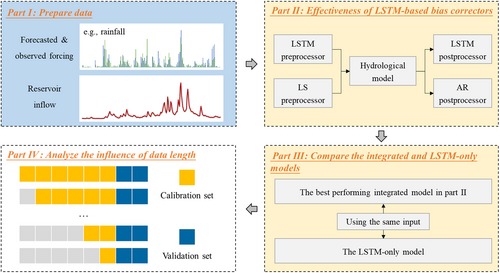
As illustrated in Figure 1, this study mainly consists of four parts:

Preparing the needed data, which includes forecasted and observed forcing (e.g., rainfall, temperature, and evaporation) and observations of reservoir inflow.
Developing and evaluating LSTM-based bias correctors for a hydrological model. The LSTM model is developed for rainfall preprocessing and inflow postprocessing, respectively. The effectiveness of the LSTM-based bias correctors is evaluated using conventional processors, that is, linear scaling (LS) and autoregressive (AR) model.
In Part III, the better performing integrated forecast model is further compared with the LSTM-based direct forecast model.
Data-driven models usually require large amounts of data for model training. However, with the continuous upgrading of climate services, consistent and long-term records of NWP data are difficult to be collected. The purpose of Part IV is to evaluate the influence of sample size on the comparison results between the integrated model and the LSTM-only model.

Details are in the caption following the image — **FIGURE 1**
Open in figure viewer PowerPoint

Framework for model development and comparison. AR, autoregressive; LS, linear scaling; LSTM, long short-term memory

2.1 LSTM network and model settings

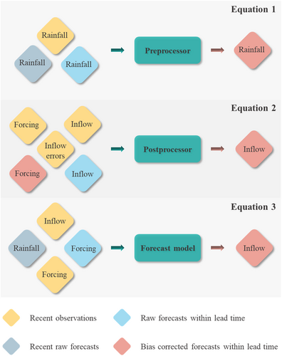
LSTM is an evolutionary version of a simple recurrent neural network, with a more elaborate design to improve the model performance under long-term dependencies (Hochreiter & Schmidhuber, 1997). All the parameters involved in LSTM cells can be learned and updated automatically according to the latent relationship between the input data and the target data. This “end-to-end” pattern endows LSTM with outstanding application value in various fields because it removes the need to manually extract the model features. In this study, LSTM-based models are used for preprocessing, postprocessing, and direct reservoir inflow forecasting. An illustration of the input and output schemes are shown in Figure 2. Blue and pink rhombuses represent raw, and bias corrected forecasts within lead time, respectively. Yellow and gray rhombuses indicate observations and raw forecasts at recent time periods, respectively.

2.1.1 Preprocessing of rainfall forecasts

To remove the inherent biases in climate model output and provide reliable estimations of rainfall uncertainty, the LSTM model is set up for preprocessing. The error characteristics of rainfall forecasts vary with lead time; therefore, the LSTM preprocessor is developed for each lead time, respectively. The input and output scheme is as follows:

P_{pre, t}^{i} = f \{\begin{cases} P_{obs, t}, P_{obs, t - 1}, \dots, P_{obs, t - l_{pre}}, \\ P_{raw, t - i}^{i}, P_{raw, t - i - 1}^{i}, \dots, P_{raw, t - i - l_{pre}}^{i}, (i = 1, 2, \dots, T) \\ P_{raw, t}^{i}, P_{raw, t}^{i - 1}, \dots, P_{raw, t}^{1} \end{cases}

(1)

where l_pre denotes the time lag used in preprocessing; T is the maximum lead time (set to 5 days in this study);

P_{obs, t}

is the observed rainfall at time t;

P_{raw, t}^{i}

and

P_{pre, t}^{i}

are the raw and preprocessed rainfall at time t + i for the lead time i, respectively.

2.1.2 Postprocessing of inflow forecasts

Inflow postprocessing relies on the autocorrelation of error series (McInerney et al., 2020; Zhang, Liu, Zhao, et al., 2018). The LSTM model is developed to correct the inflow forecasts for each lead time based on the most recent known errors, recent observation of reservoir inflow and climate forcing, and forecasted reservoir inflow and climate forcing within lead time:

Q_{fore, t}^{i} = f \{\begin{cases} e_{t}^{i}, e_{t - 1}^{i}, \dots, e_{t - l_{post}}^{i}, \\ F_{obs, t}, F_{obs, t - 1}, \dots, F_{obs, t - l_{post}}, \\ Q_{obs, t}, Q_{obs, t - 1}, \dots, Q_{obs, t - l_{post}}, (i = 1, 2, \dots, T) \\ F_{pred, t}^{i}, F_{pred, t}^{i - 1}, \dots, F_{pred, t}^{1}, \\ Q_{raw, t}^{i} {, Q}_{raw, t}^{i - 1}, \dots, Q_{raw, t}^{1} \end{cases}

(2)

where l_post denotes the time lag used in postprocessing;

e_{t}^{i}

is the inflow forecast error at time t for the lead time i;

F_{obs, t}

is the observed climate forcing at time t;

F_{pred, t}^{i}

is the bias corrected climate forcing at time t + i for the lead time i;

Q_{raw, t}^{i}

and

Q_{fore, t}^{i}

are the raw and final reservoir inflow forecasts at time t + i for the lead time i, respectively.

2.1.3 LSTM-based direct forecast model

The LSTM model is also developed as a direct predictor of reservoir inflow. Taking the same inputs as the integrated model, the LSTM-based direct forecast model is expected to learn from the latent relationship between input and target variables without prior knowledge about the bias correction-HM-bias correction process. For the forecast of the reservoir inflow at time t + i with a lead time of i, the inputs include the recent l_fore days' observation of reservoir inflow and climate forcing, raw rainfall forecasts for the time t − l_fore to t, and real-time forecasts of climate forcing within lead time. The formula is as follows:

Q_{fore, t}^{i} = f \{\begin{cases} Q_{obs, t}, Q_{obs, t - 1}, \dots, Q_{obs, t - l_{dire}}, \\ F_{obs, t}, F_{obs, t - 1}, \dots, F_{obs, t - l_{dire}}, \\ P_{raw, t}^{1 \sim i}, P_{raw, t - 1}^{1 \sim i}, \dots, P_{raw, t - l_{dire}}^{1 \sim i}, \\ F_{raw, t}^{i}, F_{raw, t}^{i - 1}, \dots, F_{raw, t}^{1}, \end{cases} (i = 1, 2, \dots, T)

(3)

where l_dire denotes the time lag used in the direct forecast;

P_{raw, t}^{1 \sim i}

represents rainfall forecasts for the time t with lead times from 1 to i;

F_{raw, t}^{i}

is the raw climate forcing from the climate model at time t + i for the lead time i.

As the learning of the LSTM model has nonnegligible randomness, several duplicate runs should be conducted. The best solution is then used for further calculations.

2.2 Benchmark processors and experimental setting

To put the LSTM models for preprocessing and postprocessing into context, benchmark preprocessing and postprocessing techniques are tested.

For preprocessing, several studies have demonstrated that the LS model is effective in correcting the bias of the climate model output (da Silva et al., 2018; Goshime et al., 2020; Ji et al., 2020). The LS is a mean-based transformation method and is easy to implement. The transformation equations are established for each grid as flows:

P_{obs}^{i} = α P_{raw}^{i}

(4)

where

P_{obs}^{i}

and

P_{raw}^{i}

are observed and raw rainfall for grid i, respectively.

To further improve the skill of inflow forecasts, forecast-based postprocessing techniques are implemented. In which postprocessing models are developed using simulations from an NWP-forced hydrological model so that the NWP and hydrological uncertainties can be simultaneously ameliorated. An AR model is selected in this study. The AR model is established for each lead time using the most recent known error (Zhang, Liu, Zhao, et al., 2018). The order of the AR model is set as two, and its parameters are determined by the modified recursive least square method.

Finally, nine forecast schemes are established (see Table 1). The schemes LS-HM, LSTM-HM, HM-AR, and HM-LSTM indicate a hydrological model combined with a preprocessor or postprocessor alone. The schemes LS-HM-AR, LS-HM-LSTM, LSTM-HM-AR, and LSTM-HM-LSTM indicate a hydrological model combined with both a preprocessor and postprocessor. The LSTM-only model means the LSTM-based direct forecast model.

TABLE 1. Forecast schemes

Forecasting methods	Schemes	Preprocessing		Hydrological modeling (HM)	Postprocessing
Forecasting methods	Schemes	LS	LSTM	Hydrological modeling (HM)	AR	LSTM
HM with bias correctors	LS-HM	√		√
	LSTM-HM		√	√
	HM-AR			√	√
	HM-LSTM			√		√
	LS-HM-AR	√		√	√
	LS-HM-LSTM	√		√		√
	LSTM-HM-AR		√	√	√
	LSTM-HM-LSTM		√	√		√
The LSTM-only model	Customized LSTM for each lead time

Abbreviations: AR, autoregressive; LS, linear scaling; LSTM, long short-term memory.

2.3 Evaluation metrics

Metrics for model evaluation include Nash–Sutcliffe efficiency (NSE) coefficient (Nash & Sutcliffe, 1970), Pearson's correlation coefficient (PCC), and bias. The percent bias in 2% high-segment flow (FHV) and 30% low-segment flow (FLV) are also calculated (Yilmaz et al., 2008). Different from Yilmaz et al. (2008), the term FLV is not calculated in the log space for the existing of flows less than or equal to zero. Only indices for the test period are presented.

2.3.1 Nash–Sutcliffe efficiency coefficient

NSE = 1 - \frac{\sum_{t = 1}^{N} {(Q_{sim, t} - Q_{obs, t})}^{2}}{\sum_{t = 1}^{N} {(Q_{obs, t} - {\bar{Q}}_{obs})}^{2}}

(5)

where

Q_{sim, t}

and

Q_{obs, t}

are the simulated and observed reservoir inflow at time t, respectively;

{\bar{Q}}_{obs}

is observed mean of reservoir inflow.

2.3.2 Pearson's correlation coefficient

PCC = \frac{\sum_{t = 1}^{N} (Q_{sim, t} - {\bar{Q}}_{sim}) (Q_{obs, t} - {\bar{Q}}_{obs})}{\sqrt{\sum_{t = 1}^{N} {(Q_{sim, t} - {\bar{Q}}_{sim})}^{2} {(Q_{obs, t} - {\bar{Q}}_{obs})}^{2}}}

(6)

where

{\bar{Q}}_{sim, t}

is the simulated mean of reservoir inflow.

2.3.3 Bias

Bias = \frac{\sum_{t = 1}^{N} (Q_{sim, t} - Q_{obs, t})}{\sum_{t = 1}^{N} Q_{obs, t}}

(7)

2.3.4 High-segment flow

FHV = \frac{\sum_{h = 1}^{H} (Q_{sim, h} - Q_{obs, h})}{\sum_{h = 1}^{H} Q_{obs, h}} \times 100

(8)

where h = 1, 2, …, H are flow indices for flows within exceedance probabilities lower than 0.02.

2.3.5 Low-segment flow

FLV = - 1 \cdot \frac{\sum_{l = 1}^{L} (Q_{sim, l} - Q_{sim, L}) - \sum_{l = 1}^{L} (Q_{obs, l} - Q_{obs, L})}{\sum_{l = 1}^{L} (Q_{obs, l} - Q_{obs, L})} \times 100

(9)

where l = 1, 2, …, L are flow indices for flows with exceedance probabilities greater than 0.7; L is the index for the minimum flow.

3 CASE STUDIES

Two case studies are conducted to illustrate the role of the LSTM model in improving the accuracy of reservoir inflow forecasting. The location of the reservoirs, used data, and rainfall-runoff models are presented in this section.

3.1 Location

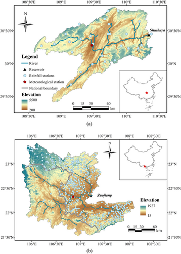
Figure 3 presents the location of the Shuibuya and Zuojiang reservoirs. The Shuibuya reservoir is located in Hubei province, China. As the first cascade in the mainstream of Qingjiang River, a branch of the Yangtze River, the main operational purposes of this dam are flood control and power generation. The drainage area that contributes to the Shuibuya reservoir inflow covers 10,860 km², accounting for 64% of the whole watershed. Qingjiang river basin has a subtropical monsoon climate. Some 80% of the annual rainfall occurs from April to September. Storm flood events are frequent because of the complex climate and topography, threatening local security and the economy. Therefore, accurate reservoir inflow forecasting is desperately needed. The Zuojiang reservoir has a drainage area of 26,173 km² and is located in the middle reaches of the Zuojiang river. The dam is primarily used for hydropower generation and has comprehensive utilization benefits such as irrigation, shipping, tourism, and aquaculture. The Zuojiang river, with a total length of 539 km, is a transborder river whose upper reaches belong to Vietnam (about 40% of the drainage area of the Zuojiang reservoir), and the middle and lower reaches belong to China.

3.2 Data and HM

3.2.1 Shuibuya reservoir

The available data for this area consists of reservoir inflows to Shuibuya reservoir, rainfall, and maximum/minimum temperatures, all of which were obtained for the period 2014–2019. These years include relatively dry, normal, and wet conditions. The reservoir inflows, which are calculated through the inversion of the water balance function based on the observed reservoir level and outflows, were obtained from the operator of the Shuibuya reservoir. The meteorological data were recorded at the gage stations shown in Figure 3. Rainfall data were collected from the operator of the Shuibuya reservoir, and temperature data were obtained from the National Meteorological Information Center, China (http://data.cma.cn). After considering the time difference between weather predictions, all the obtained data were converted to daily time scales to satisfy the forecasting objectives of this research.

Real-time NWP data were obtained from the National Centers for Environmental Prediction, America (NCEP). The NCEP operational Global Forecast System gives global 16-day forecasts on a 0.25° spatial scale (about 30 km horizontal resolution) every 6 h from January 15, 2015, to the current time (https://rda.ucar.edu/datasets/ds084.1/). The first 10 days of forecasts are given at 3-h intervals, with subsequent predictions given at 12-h intervals. The first 5 days of forecasts are used in this study as the errors of weather predictions increase with the growth of lead time.

Generally, a climate model and a distributed hydrological model are combined for modeling the runoff processes. This is because the climate model outputs fit well with the gridded form of the distributed hydrological model inputs. The macroscale variable infiltration capacity (VIC) distributed hydrological model (Liang et al., 1994) is chosen to simulate the reservoir inflow. The model runs at a 0.25° grid spatial scale, including inputs of the rainfall and the maximum/minimum temperatures. The calibration and validation of the VIC model are detailed in Appendix A.

3.2.2 Zuojiang reservoir

Hourly observed data, including reservoir inflow and rainfall, and daily rainfall forecasts are obtained from January 2013 to October 2020. These data are collected from the operator of this dam. The estimated reservoir inflow, using the water balance method, is regarded as the “observed” inflow. The rainfall forecasts are issued every 12 h by the Guangxi Zhuang Autonomous Region Meteorological Bureau, China, and have a forecast horizon of 5 days. Both the observed and forecasted rainfall is given as an average. The conceptual rainfall-runoff model Xinanjiang (Zhao, 1992), which has been widely used for humid catchments in China, is selected to simulate the reservoir inflow. Besides, running a Xinanjiang model requires both rainfall and evapotranspiration (ET) data. Daily ET from 2013 to 2019 was downloaded from the National Meteorological Information Center (http://data.cma.cn). To fill the gaps of different time spans between rainfall and ET and lacking of ET forecasts, the ET data are averaged to 1 year because that ET has relatively little influence on reservoir inflow. Then, each year shares the same ET when running the Xinanjiang model. The calibration and validation of the Xinanjiang (XAJ) model are detailed in Appendix A.

4 FORECAST RESULTS AND DISCUSSIONS

4.1 Effectiveness of LSTM-based bias correctors

To demonstrate the effectiveness of LSTM-based bias correctors, a total of eight schemes are obtained by considering the configurations of HM with only a preprocessor, postprocessor, and both Table 2 and Table 3 present the forecast results for Shuibuya and Zuojiang reservoirs, respectively.

TABLE 2. Shuibuya: Performance of variable infiltration capacity (VIC) model with different processing scheme for multi-step ahead reservoir inflow forecast

Metrics	Lead time (day)	Schemes
Metrics	Lead time (day)	LS-VIC	LSTM-VIC	VIC-AR	VIC-LSTM	LS-VIC-AR	LS-VIC-LSTM	LSTM-VIC-AR	LSTM-VIC-LSTM
NSE	t + 1	0.65	0.66	0.50	0.82	0.71	0.84	0.74	0.84
	t + 2	0.57	0.59	0.22	0.70	0.58	0.72	0.61	0.72
	t + 3	0.54	0.53	0.02	0.57	0.55	0.61	0.55	0.66
	t + 4	0.40	0.43	−0.31	0.52	0.40	0.55	0.44	0.58
	t + 5	0.29	0.40	−0.76	0.44	0.29	0.45	0.40	0.47
PCC	t + 1	0.82	0.81	0.81	0.91	0.85	0.92	0.86	0.92
	t + 2	0.78	0.77	0.76	0.84	0.78	0.86	0.79	0.86
	t + 3	0.76	0.73	0.74	0.76	0.77	0.80	0.75	0.82
	t + 4	0.68	0.67	0.65	0.77	0.68	0.76	0.68	0.79
	t + 5	0.63	0.65	0.58	0.68	0.63	0.67	0.65	0.73
Bias	t + 1	0.07	−0.03	0.16	−0.07	0.05	0.02	−0.02	0.02
	t + 2	0.10	−0.05	0.30	0.04	0.09	−0.04	−0.04	−0.03
	t + 3	0.11	−0.08	0.36	−0.04	0.10	0.07	−0.07	0.10
	t + 4	0.12	−0.12	0.43	−0.04	0.12	−0.12	−0.13	0.00
	t + 5	0.12	−0.13	0.48	0.01	0.12	−0.03	−0.13	0.09
FHV	t + 1	−0.21	−0.29	−0.13	−0.11	−0.19	−0.07	−0.23	−0.07
	t + 2	−0.27	−0.37	−0.14	−0.14	−0.28	−0.15	−0.36	−0.12
	t + 3	−0.27	−0.43	−0.25	−0.42	−0.28	−0.26	−0.43	−0.17
	t + 4	−0.40	−0.56	−0.22	−0.25	−0.40	−0.33	−0.56	−0.18
	t + 5	−0.41	−0.55	−0.67	−0.43	−0.41	−0.56	−0.54	−0.35
FLV	t + 1	−0.20	−0.02	−0.24	−0.08	−0.22	−0.39	−0.21	−0.39
	t + 2	−0.30	−0.04	−0.39	−0.27	−0.28	−0.22	−0.08	−0.21
	t + 3	−0.40	−0.08	−0.26	−0.52	−0.29	−0.38	−0.15	−0.60
	t + 4	−0.49	−0.05	−0.35	0.32	−0.42	0.39	0.00	−0.38
	t + 5	−0.53	−0.07	−0.42	−0.29	−0.51	−0.72	−0.08	−0.47

Note: Bold text corresponds to the best-performing scheme.
Abbreviations: AR, autoregressive; FHV, high-segment flow; FLV, low-segment flow; LS, linear scaling; LSTM, long short-term memory; NSE, Nash–Sutcliffe efficiency; PCC, Pearson's correlation coefficient.

TABLE 3. Zuojiang: Performance of Xinanjiang (XAJ) model with different processing scheme for multi-step ahead reservoir inflow forecast

Metrics	Lead time (day)	Schemes
Metrics	Lead time (day)	LS-XAJ	LSTM-XAJ	XAJ-AR	XAJ-LSTM	LS-XAJ-AR	LS-XAJ-LSTM	LSTM-XAJ-AR	LSTM-XAJ-LSTM
NSE	t + 1	0.64	0.64	0.90	0.96	0.90	0.96	0.90	0.96
	t + 2	0.59	0.59	0.70	0.88	0.70	0.87	0.70	0.88
	t + 3	0.49	0.49	0.53	0.80	0.53	0.80	0.51	0.79
	t + 4	0.42	0.40	0.42	0.70	0.44	0.72	0.41	0.73
	t + 5	0.39	0.36	0.39	0.67	0.42	0.68	0.39	0.69
PCC	t + 1	0.87	0.87	0.95	0.98	0.95	0.98	0.96	0.98
	t + 2	0.83	0.83	0.86	0.94	0.86	0.93	0.86	0.94
	t + 3	0.78	0.76	0.80	0.89	0.78	0.90	0.77	0.89
	t + 4	0.73	0.69	0.75	0.84	0.73	0.85	0.70	0.85
	t + 5	0.70	0.65	0.72	0.83	0.71	0.83	0.67	0.82
Bias	t + 1	0.17	0.17	0.03	−0.03	0.03	0.04	0.03	0.01
	t + 2	0.15	0.14	0.05	−0.01	0.04	−0.03	0.04	−0.05
	t + 3	0.12	0.10	0.06	−0.01	0.05	0.01	0.04	−0.01
	t + 4	0.09	0.05	0.08	−0.09	0.05	0.06	0.02	−0.04
	t + 5	0.05	0.01	0.07	−0.02	0.02	0.06	−0.02	0.04
FHV	t + 1	−0.07	−0.08	−0.01	0.02	−0.01	0.02	−0.01	0.00
	t + 2	−0.17	−0.18	−0.15	−0.16	−0.15	−0.14	−0.15	−0.11
	t + 3	−0.31	−0.34	−0.27	−0.29	−0.31	−0.24	−0.34	−0.29
	t + 4	−0.38	−0.46	−0.32	−0.28	−0.38	−0.29	−0.46	−0.27
	t + 5	−0.46	−0.56	−0.40	−0.32	−0.45	−0.34	−0.54	−0.33
FLV	t + 1	−5.35	−5.35	0.06	−0.65	0.06	−0.18	0.06	0.30
	t + 2	−5.25	−5.27	0.24	0.01	0.28	0.18	0.30	0.02
	t + 3	−5.29	−5.35	0.37	−0.33	0.44	−0.86	0.46	−0.31
	t + 4	−5.39	−5.47	0.32	−0.25	0.31	−0.94	0.28	−0.14
	t + 5	−5.50	−5.60	0.26	−0.28	0.29	−0.33	0.29	−0.79

Note: Bold text corresponds to the best-performing scheme.
Abbreviations: AR, autoregressive; FHV, high-segment flow; FLV, low-segment flow; LS, linear scaling; LSTM, long short-term memory; NSE, Nash–Sutcliffe efficiency; PCC, Pearson's correlation coefficient.

The scores are generally better when the preprocessing and postprocessing technique are jointly implemented, which suggests that both the rainfall and hydrological uncertainty should be considered in hydrometeorological forecasting. However, the relative importance of preprocessing and postprocessing is not consistent in the two cases, which depend strongly on the selected models and research objects (Sharma et al., 2018). Within the preprocessing methods, the LSTM-based preprocessor corrects the bias in rainfall forecasts more effectively (detailed in Appendix B). The LS is a mean-based correction technique, which removes systematic bias in rainfall forecasts, while the relationship between the observations and forecasts is not simply linear. Nonetheless, there are also some cases in which the LS preprocessor makes the inflow forecasts more accurate. For instance, the scheme LS-XAJ provides better 4–5 days-ahead forecasts than LSTM-XAJ (Table 3). This is understandable because uncertainties from the hydrological model are included in the evaluation when the observed reservoir inflow is used as the benchmark. For postprocessing, the AR model corrects inflow forecasts effectively and produces consistent improvements for both reservoirs and all lead times. The gains in NSE value from AR vary from 0 to 0.06 and 0 to 0.26 for Shuibuya and Zuojiang reservoirs, respectively. The improvements seem to be larger at the shorter lead times. Using the same input, schemes with an LSTM postprocessor give further improvements in NSE, which range from 0.06 to 0.31. Skill improvements are also observed in terms of PCC, Bias, FLV, and FHV. The schemes with both an LSTM-based preprocessor and postprocessor perform best among all the schemes, although the differences are not significant in some cases, for example, scheme XAJ-LSTM versus LSTM-XAJ-LSTM for 4 days ahead forecasts of Zuojiang reservoir. Importantly, the LSTM-based bias correctors provide consistent improvements for preprocessing and postprocessing across lead times.

4.2 Comparison of the hybrid and LSTM-only models

This subsection examines whether a process-based model with bias correctors or a pure data-driven model performs better in multi-step ahead reservoir inflow forecasts. Figure 4 (Shuibuya) and Figure 5 (Zuojiang) illustrate the skill indices of the better-performing integrated scheme, that is, HM with LSTM correctors and the customized LSTM model for each lead time.

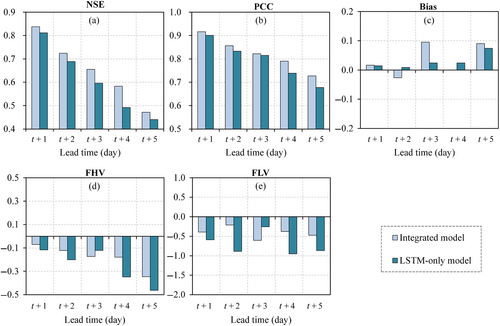
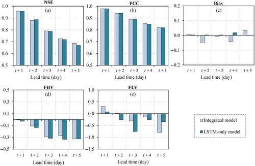
For the Shuibuya reservoir, the integrated model provides better scores across lead times. The NSE value (Figure 4a) decreases from 0.84 to 0.47 and 0.81 to 0.44 for the integrated model and LSTM-only model, respectively. The discrepancies in NSE value between the two paradigms range from 0.03 to 0.06, indicating that slight improvements can be obtained by using the integrated model. Similar results are obtained for the metrics of PCC, FHV, and FLV. Besides, the bias of the two models is within 10% for all lead times.

For the Zuojiang reservoir, however, there are no significant differences between the integrated model and the LSTM-only model. The NSE value for the integrated model is 0.96 at 1 day ahead forecast, and it drops to 0.69 at 5 days ahead forecast. For the LSTM-only model, the NSE value ranges from 0.96 to 0.67 for forecasts from one to 5 days ahead. The discrepancies in the NSE value are lower than 0.02, which can be attributed to the randomness in the training process (Gauch et al., 2021). The results of the other four metrics also show that the integrated model produces comparable forecasts with the LSTM-only model.

Figure 6 displays two typical flood events of the Shuibuya reservoir. The 1, 3, and 5 day(s) ahead forecasts are presented separately. The integrated and LSTM-only models performed similarly for the one-day ahead forecasts. Both models underestimated the flood peak of flood event 20,180,506 while overestimated the flood peak of flood event 20,180,706. It can be observed that the rainfall was overestimated for the two flood events. The overestimation of the flood peak can be easily attributed to the overestimations in rainfall forecasts, and the underestimation of the flood peak may be caused by other factors, for example, incorrect forecast of the temporal and spatial distribution of rainfall. For the 3 days ahead forecasts, the two models give close results for the flood event 20,180,506. However, the integrated model performs better for the forecasting of the flood event 20,180,706. The NSE value of the integrated model is 0.26 higher than the LSTM-only model for its better capturing of the flood peak. When the lead time grows to 5 days (Figures 5f and 6e), both the integrated and LSTM-only models struggle to capture the flood. The two models wrongly forecasted the timing of the flood peak for both flood events, which is consistent with the bias in rainfall forecasts.

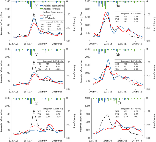
Figure 7 describes the forecasts for the Zuojiang reservoir. For the flood event 20,190,805, the integrated and LSTM-only models provide similar and accurate forecasts for 1, 3, and 5 days ahead, with the NSE value greater than 0.90. For the flood event 20,201,016, both models produced accurate forecasts for 1 day ahead. The LSTM-only model underestimated the flood peak in 3 days ahead forecasts, while the integrated model underestimated the flood peak in 5 days ahead forecasts. These underestimations may be attributed to the underestimations in rainfall forecasts because the reservoir inflow with a longer lead time is less related to the most recent inflow observations but highly related to rainfall forecasts.

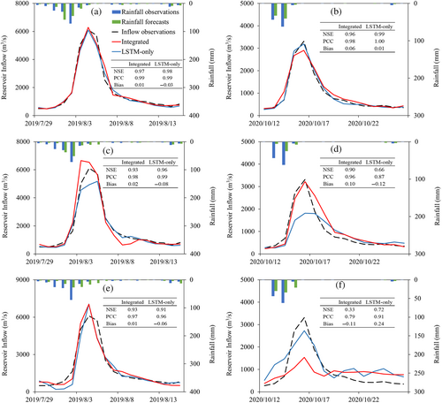
From the analyses above, it can be found that the integrated model provides better inflow forecasts of the Shuibuya reservoir than the LSTM-only model. These improvements are significant in statistics, with the discrepancy in NSE value ranging from 0.03 to 0.06, but not translated into practical improvements in flood hydrographs. For the Zuojiang reservoir, the integrated model and LSTM-only model show similar performance in evaluation metrics and flood hydrographs.

4.3 Influence of data length

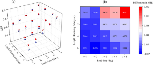
The forecast results of the Shuibuya and Zuojiang reservoirs lead to different conclusions about the comparison of the integrated model and LSTM-only model. It is generally accepted that the length of training data has a significant influence on the performance of data-driven models. However, the length of the collected data of the Shuibuya reservoir is different from that of the Zuojiang reservoir. The data length of Shuibuya reservoir is 5 years (3 years data for model training), while the data length of Zuojiang reservoir is 8 years (6 years data for model training). Therefore, the influence of the data length must be considered. Taking Zuojiang reservoir as the testbed, the integrated model and LSTM-only model are trained with varying lengths of data, for example, 1, 2, 4, and 6 years, and the model performances are evaluated with the data of the last 2 years.

The comparison results are presented in Figure 8. Figure 8a depicts the NSE value of the integrated model and LSTM-only model under different lengths of training data and lead times. It can be found that the performance of the LSTM-only model decreases rapidly due to under-fitting, while the integrated model provides more robust forecasts under varying data lengths. The differences in NSE value (Figure 8b) between the two models become larger at the long lead times. This means that explicitly considering a rainfall preprocessing, rainfall-runoff modeling, and inflow postprocessing process is helpful for multi-step ahead reservoir inflow forecast. A well-calibrated rainfall-runoff model can reasonably represent the reservoir inflow process under specific initial conditions and predicted weather conditions. The errors of inflow forecasts mainly originate from the uncertainties in rainfall forecasts and defects of the rainfall-runoff model. The forecasting quality can be effectively improved if the two types of errors are corrected. For the LSTM-only model, there is no such a process guide. With increasing uncertainties in rainfall forecasts and decreasing useful information abstracted from recent observations as lead time grows, it becomes harder for the LSTM-only model to capture the latent relationship between input and output data. However, increasing the length of training data can greatly narrow the accuracy gap between the integrated and LSTM-only models; similar conclusions were drawn by Wang et al. (2019). For 5 days ahead forecasts, the difference in NSE value decreases from 0.11 to 0.02 when the length of training data grows from 1 to 6 years.

5 CONCLUSIONS

In this study, the role of the LSTM model in multi-step ahead reservoir inflow forecast was investigated by considering the integrated model (using the LSTM model as a bias corrector for a hydrological model) and LSTM-only models. First, the effectiveness of LSTM-based correctors in preprocessing and postprocessing is assessed by comparing them with conventional processors. Second, the performance of the integrated model and LSTM-only models is analyzed. Two reservoirs were taken as examples. The main conclusions are as follows:

LSTM models for bias correction are effective in both preprocessing and postprocessing. In preprocessing, the LSTM corrector is superior to the linear transformation method, with lower root mean square error (RMSE) and higher PCC score. For postprocessing, the gains in NSE value from AR vary from 0 to 0.06 and 0 to 0.26 for Shuibuya and Zuojiang reservoirs, respectively. Using the same input, the LSTM postprocessor gives further improvements in NSE, which range from 0.06 to 0.31.
The integrated model provides better results than the LSTM-only model in the Shuibuya reservoir, while it is comparable to the LSTM-only model in the Zuojiang reservoir. For the Shuibuya reservoir, slight improvements can be obtained by using the integrated model, with the discrepancy in NSE value ranging from 0.03 to 0.06. For the Zuojiang reservoir, the discrepancies in NSE value are lower than 0.02, which can be attributed to the randomness in the training process. Furthermore, with the Zuojiang reservoir as a testbed, the two types of models are trained with varying data lengths. The integrated model is comparable to the LSTM-only when trained with more than 4 years of data, while it is better than the LSTM-only under limited data, especially for the longer lead time. The difference in NSE value for 5 days ahead forecasts increases from 0.02 to 0.11 when the length of training data decreases from 6 to 1 year. This indicates that the length of training data has a significant influence on the integrated model and LSTM-only model.

This study demonstrated the efficacy of a rainfall-runoff model with LSTM-based bias correctors for flood forecasting, which is valuable for flood risk mitigation. However, some points need to be further investigated. The conclusions of this study can be verified at more catchments. Besides, with the continuous upgrading of climate services, it is difficult to collect consistent and long-term records of NWP data, which may limit the accuracy of the flood forecasting. One potential way to mitigate this problem is to develop a global LSTM model (Kratzert et al., 2018; Kratzert et al., 2019). At last, the conclusions emphasize the understanding of each part of the modeling chain, which implies that the performance of the LSTM model and other data-driven models may be improved by including the human cognition of physical processes, especially when limited data can be obtained.

ACKNOWLEDGMENTS

This study was supported by the Joint Funds of the National Natural Science Foundation of China (Grant No. U1865201), National Natural Science Foundation of China (Grant No. 51861125102), and Innovation Team in Key Field of the Ministry of Science and Technology (Grant No. 2018RA4014).

CONFLICT OF INTEREST

The authors declare that they have no known competing financial interests or personal relationships that could have appeared to influence the work reported in this paper.

APPENDIX A

A.1 Hydrological modeling

A.1.1. Shuibuya reservoir

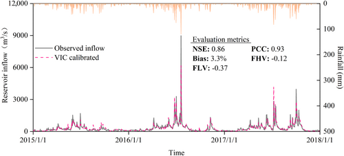
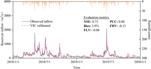
The VIC model was established at a daily time scale and 0.25° spatial scale. To ensure a consistent time span of data for the calibration of VIC and LSTM models, data for the year 2014 were used to warm up the VIC model, while the data for 2015–2017 were used as the calibration period, and the remainder was used as the validation period. The simulated reservoir inflow and evaluation indices are presented in Figures A1 and A2.

A.1.2. Zuojiang reservoir

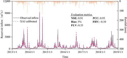
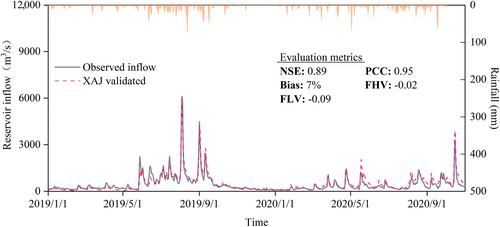
The daily XAJ model was calibrated in the period from 2013 to 2018 (including a 60 days warmup period) and validated in 2019–2020. Figures A3 and A4 present the observed and simulated inflow. The XAJ model performs well in both periods, with the NSE value close to 0.9. However, the rain gauges cover only the area in China, making the inflow simulations show significant error during some periods. For instance, the floods in 2015 and 2018.

APPENDIX B

B.1 NWP performance evaluation

The rainfall forecasts are corrected by using LS and LSTM methods. A distributed hydrological model is established for Shuibuya reservoir; the LS method corrects the bias in rainfall forecast grid by grid, while the LSTM method corrects the gridded rainfall forecasts synchronously. Table B1 shows the metrics of the raw and bias-corrected rainfall forecasts for the Shuibuya and Zuojiang reservoirs. The evaluation was performed at the catchment scale. For both reservoirs, preprocessing techniques can effectively correct the bias in the rainfall forecasts, giving lower RMSE values. The LSTM-based method also gives some improvements in terms of PCC by considering non-linear relationships within input and output data.

TABLE B1. Metrics of the raw and preprocessed rainfall for 1–5 days ahead

Reservoir	Methods	Metrics	t + 1	t + 2	t + 3	t + 4	t + 5
Shuibuya	Raw	RMSE	5.32	7.18	8.35	9.19	8.75
	Raw	PCC	0.78	0.69	0.62	0.51	0.48
	LS	RMSE	4.26	5.11	5.76	6.36	6.38
	LS	PCC	0.78	0.69	0.62	0.51	0.48
	LSTM	RMSE	4.03	4.66	5.16	5.56	5.75
	LSTM	PCC	0.79	0.71	0.62	0.53	0.48
Zuojiang	Raw	RMSE	5.72	6.07	6.23	6.59	6.70
	Raw	PCC	0.74	0.70	0.67	0.62	0.60
	LS	RMSE	5.59	5.96	6.23	6.58	6.70
	LS	PCC	0.74	0.70	0.67	0.62	0.60
	LSTM	RMSE	5.44	5.80	6.19	6.48	6.54
	LSTM	PCC	0.76	0.73	0.68	0.63	0.63

Abbreviations: LS, linear scaling; LSTM, long short-term memory; PCC, Pearson's correlation coefficient; RMSE, root mean square error.

Open Research

DATA AVAILABILITY STATEMENT

(1) Real-time numerical weather prediction data for the Shuibuya reservoir were obtained from NCEP (https://rda.ucar.edu/datasets/ds084.1/). Other rainfall data are collected from the operators of the dams, with agreements requirement for use, and are not accessible to the public or research community directly. (2) Daily maximum/minimum temperatures and ET data were obtained from the National Meteorological Information Center (http://data.cma.cn). (3) All models or codes that support the findings of this study are available from the corresponding author upon reasonable request.

REFERENCES

Ahmad, S. K., & Hossain, F. (2020). Maximizing energy production from hydropower dams using short-term weather forecasts. Renewable Energy, 146, 1560–1577. https://doi.org/10.1016/j.renene.2019.07.126
10.1016/j.renene.2019.07.126
Web of Science® Google Scholar
Ahmad, S. K., & Hussain, F. (2019). A generic data-driven technique for forecasting of reservoir inflow: Application for hydropower maximization. Environmental Modelling & Software, 119, 147–165. https://doi.org/10.1016/j.envsoft.2019.06.008
10.1016/j.envsoft.2019.06.008
Web of Science® Google Scholar
Anghileri, D., Monhart, S., Zhou, C., Bogner, K., Castelletti, A., Burlando, P., & Zappa, M. (2019). The value of subseasonal hydrometeorological forecasts to hydropower operations: How much does preprocessing matter. Water Resources Research, 55(12), 10159–10178. https://doi.org/10.1029/2019WR025280
10.1029/2019WR025280
Web of Science® Google Scholar
Anghileri, D., Voisin, N., Castelletti, A., Pianosi, F., Nijssen, B., & Lettenmaier, D. P. (2016). Value of long-term streamflow forecasts to reservoir operations for water supply in snow-dominated river catchments. Water Resources Research, 52(6), 4209–4225. https://doi.org/10.1002/2015WR017864
10.1002/2015WR017864
Web of Science® Google Scholar
Bauer, P., Thorpe, A., & Brunet, G. (2015). The quiet revolution of numerical weather prediction. Nature, 525(7567), 47–55. https://doi.org/10.1038/nature14956
10.1038/nature14956
CAS PubMed Web of Science® Google Scholar
Bennett, J. C., Robertson, D. E., Shrestha, D. L., Wang, Q. J., Enever, D., Hapuarachchi, P., & Tuteja, N. K. (2014). A system for continuous hydrological ensemble forecasting (SCHEF) to lead times of 9 days. Journal of Hydrology, 519, 2832–2846. https://doi.org/10.1016/j.jhydrol.2014.08.010
10.1016/j.jhydrol.2014.08.010
Web of Science® Google Scholar
Benninga, H.-J. F., Booij, M. J., Romanowicz, R. J., & Rientjes, T. H. M. (2017). Performance of ensemble streamflow forecasts under varied hydrometeorological conditions. Hydrology and Earth System Sciences, 21(10), 5273–5291. https://doi.org/10.5194/hess-21-5273-2017
10.5194/hess-21-5273-2017
Web of Science® Google Scholar
da Silva, F. D. N. R., Alves, J. L. D., & Cataldi, M. (2018). Climate downscaling over South America for 1971–2000: Application in SMAP rainfall-runoff model for Grande River basin. Climate Dynamics, 52, 681–696. https://doi.org/10.1007/s00382-018-4166-7
10.1007/s00382-018-4166-7
Web of Science® Google Scholar
Deng, C., Liu, P., Liu, Y., Wu, Z., & Wang, D. (2015). Integrated hydrologic and reservoir routing model for real-time water level forecasts. Journal of Hydrologic Engineering, 20(9), 05014032. https://doi.org/10.1061/(asce)he.1943-5584.0001138
10.1061/(asce)he.1943-5584.0001138
Web of Science® Google Scholar
Feng, D., Fang, K., & Shen, C. (2020). Enhancing streamflow forecast and extracting insights using long-short term memory networks with data integration at continental scales. Water Resources Research, 56(9), e2019WR026793. https://doi.org/10.1029/2019wr026793
10.1029/2019wr026793
Web of Science® Google Scholar
Fernández Bou, A. S., De Sá, R. V., & Cataldi, M. (2015). Flood forecasting in the upper Uruguay River basin. Natural Hazards, 79(2), 1239–1256. https://doi.org/10.1007/s11069-015-1903-7
10.1007/s11069-015-1903-7
Web of Science® Google Scholar
Gauch, M., Mai, J., & Lin, J. (2021). The proper care and feeding of CAMELS: How limited training data affects streamflow prediction. Environmental Modelling & Software, 135, 104926. https://doi.org/10.1016/J.ENVSOFT.2020.104926
10.1016/J.ENVSOFT.2020.104926
Web of Science® Google Scholar
Georgakakos, K. P., Graham, N. E., Modrick, T. M., Murphy, M. J., Shamir, E., Spencer, C. R., & Sperfslage, J. A. (2014). Evaluation of real-time hydrometeorological ensemble prediction on hydrologic scales in northern California. Journal of Hydrology, 519, 2978–3000. https://doi.org/10.1016/j.jhydrol.2014.05.032
10.1016/j.jhydrol.2014.05.032
Web of Science® Google Scholar
Gong, Y., Liu, P., Zhang, J., Liu, D., Zhang, X., & Zhang, X. (2020). Considering different streamflow forecast horizons in the quantitative flood risk analysis for a multi-reservoir system. Reliability Engineering and System Safety, 204, 107128. https://doi.org/10.1016/j.ress.2020.107128
10.1016/j.ress.2020.107128
Web of Science® Google Scholar
Goshime, D. W., Absi, R., Haile, A. T., Ledesert, B., & Rientjes, T. (2020). Bias-corrected CHIRP satellite rainfall for water level simulation, Lake Ziway, Ethiopia. Journal of Hydrologic Engineering, 25(9), 05020024. https://doi.org/10.1061/(ASCE)HE.1943-5584.0001965
10.1061/(ASCE)HE.1943-5584.0001965
Web of Science® Google Scholar
Gui, Z., Liu, P., Cheng, L., Guo, S., Wang, H., & Zhang, L. (2019). Improving runoff prediction using remotely sensed actual evapotranspiration during rainless periods. Journal of Hydrologic Engineering, 24(12), 04019050. https://doi.org/10.1061/(ASCE)HE.1943-5584.0001856
10.1061/(ASCE)HE.1943-5584.0001856
Web of Science® Google Scholar
Hochreiter, S., & Schmidhuber, J. (1997). Long short-term memory. Neural Computation, 9(8), 1735–1780. https://doi.org/10.1162/neco.1997.9.8.1735
10.1162/neco.1997.9.8.1735
CAS PubMed Web of Science® Google Scholar
Ji, X., Li, Y. G., Luo, X., He, D. M., Guo, R. Y., Wang, J., Bai, Y., Yue, C. Y., & Liu, C. (2020). Evaluation of bias correction methods for APHRODITE data to improve hydrologic simulation in a large Himalayan basin. Atmospheric Research, 242, 104964. https://doi.org/10.1016/j.atmosres.2020.104964
10.1016/j.atmosres.2020.104964
Web of Science® Google Scholar
Jiang, S., Zheng, Y., & Solomatine, D. (2020). Improving AI system awareness of geoscience knowledge: Symbiotic integration of physical approaches and deep learning. Geophysical Research Letters, 47(13), e2020GL088229. https://doi.org/10.1029/2020gl088229
10.1029/2020gl088229
Web of Science® Google Scholar
Kao, I. F., Zhou, Y., Chang, L.-C., & Chang, F.-J. (2020). Exploring a long short-term memory based encoder-decoder framework for multi-step-ahead flood forecasting. Journal of Hydrology, 583, 124631. https://doi.org/10.1016/j.jhydrol.2020.124631
10.1016/j.jhydrol.2020.124631
Web of Science® Google Scholar
Kratzert, F., Klotz, D., Brenner, C., Schulz, K., & Herrnegger, M. (2018). Rainfall–runoff modelling using long short-term memory (LSTM) networks. Hydrology and Earth System Sciences, 22(11), 6005–6022. https://doi.org/10.5194/hess-22-6005-2018
10.5194/hess-22-6005-2018
Web of Science® Google Scholar
Kratzert, F., Klotz, D., Shalev, G., Klambauer, G., Hochreiter, S., & Nearing, G. (2019). Towards learning universal, regional, and local hydrological behaviors via machine learning applied to large-sample datasets. Hydrology and Earth System Sciences, 23(12), 5089–5110. https://doi.org/10.5194/hess-23-5089-2019
10.5194/hess-23-5089-2019
Web of Science® Google Scholar
Li, H., Liu, P., Guo, S., Ming, B., Cheng, L., & Zhou, Y. (2018). Hybrid two-stage stochastic methods using scenario-based forecasts for reservoir refill operations. Journal of Water Resources Planning and Management, 144(12), 04018080. https://doi.org/10.1061/(ASCE)WR.1943-5452.0001013
10.1061/(ASCE)WR.1943-5452.0001013
Web of Science® Google Scholar
Liang, X., Lettenmaier, D. P., Wood, E. F., & Burges, S. J. (1994). A simple hydrologically based model of land-surface water and energy fluxes for general-circulation models. Journal of Geophysical Research-Atmospheres, 99(D7), 14415–14428. https://doi.org/10.1029/94JD00483
10.1029/94JD00483
Web of Science® Google Scholar
Liao, S. L., Liu, Z. W., Liu, B. X., Cheng, C. T., Jin, X. F., & Zhao, Z. P. (2020). Multistep-ahead daily inflow forecasting using the ERA-interim reanalysis data set based on gradient-boosting regression trees. Hydrology and Earth System Sciences, 24(5), 2343–2363. https://doi.org/10.5194/hess-24-2343-2020
10.5194/hess-24-2343-2020
Web of Science® Google Scholar
Liu, G. B., Zhou, J. Z., Yang, Y. Q., Ke, S. L., Mo, L., Wang, Y. Q., & Xiao, X. G. (2020). Risks analysis of discarding water in power generation process of hydropower station. IEEE Access, 8, 132703–132720. https://doi.org/10.1109/ACCESS.2019.2931939
10.1109/ACCESS.2019.2931939
Web of Science® Google Scholar
Liu, P., Li, L. P., Guo, S. L., Xiong, L. H., Zhang, W., Zhang, J. W., & Xu, C. Y. (2015). Optimal design of seasonal flood limited water levels and its application for the Three Gorges Reservoir. Journal of Hydrology, 527, 1045–1053. https://doi.org/10.1016/j.jhydrol.2015.05.055
10.1016/j.jhydrol.2015.05.055
Web of Science® Google Scholar
Liu, P., Zhang, X., Zhao, Y., Deng, C., Li, Z., & Xiong, M. (2018). Improving efficiencies of flood forecasting during lead times: An operational method and its application in the Baiyunshan Reservoir. Hydrology Research, 50(2), 709–724. https://doi.org/10.2166/nh.2018.051
10.2166/nh.2018.051
Web of Science® Google Scholar
Liu, X. L., & Coulibaly, P. (2011). Downscaling ensemble weather predictions for improved week-2 hydrologic forecasting. Journal of Hydrometeorology, 12(6), 1564–1580. https://doi.org/10.1175/2011JHM1366.1
10.1175/2011JHM1366.1
Web of Science® Google Scholar
Lu, X. C., Sha, Y. H., Li, Z. N., Huang, Y. Q., Chen, W. Y., Chen, D. H., Shen, J., Chen, Y., & Fung, J. C. H. (2021). Development and application of a hybrid long-short term memory—Three dimensional variational technique for the improvement of PM2.5 forecasting. Science of the Total Environment, 770, 144221. https://doi.org/10.1016/j.scitotenv.2020.144221
10.1016/j.scitotenv.2020.144221
CAS PubMed Web of Science® Google Scholar
Ma, J., Ding, Y. X., Cheng, J. C. P., Jiang, F. F., & Wan, Z. W. (2019). A temporal-spatial interpolation and extrapolation method based on geographic long short-term memory neural network for PM2.5. Journal of Cleaner Production, 237, 117729. https://doi.org/10.1016/j.jclepro.2019.117729
10.1016/j.jclepro.2019.117729
CAS Web of Science® Google Scholar
McInerney, D., Thyer, M., Kavetski, D., Laugesen, R., Tuteja, N., & Kuczera, G. (2020). Multi-temporal hydrological residual error modelling for seamless subseasonal streamflow forecasting. Water Resources Research, 57, e2019WR026979. https://doi.org/10.1029/2019WR026979
10.1029/2019WR026979
Web of Science® Google Scholar
Miao, Y. B., Chen, X. D., & Hossain, F. (2016). Maximizing hydropower generation with observations and numerical modeling of the atmosphere. Journal of Hydrologic Engineering, 21(6), 02516002. https://doi.org/10.1061/(ASCE)HE.1943-5584.0001405
10.1061/(ASCE)HE.1943-5584.0001405
Web of Science® Google Scholar
Monhart, S., Zappa, M., Spirig, C., Schär, C., & Bogner, K. (2019). Subseasonal hydrometeorological ensemble predictions in small- and medium-sized mountainous catchments: Benefits of the NWP approach. Hydrology and Earth System Sciences, 23(1), 493–513. https://doi.org/10.5194/hess-23-493-2019
10.5194/hess-23-493-2019
Web of Science® Google Scholar
Nanda, T., Sahoo, B., & Chatterjee, C. (2019). Enhancing real-time streamflow forecasts with wavelet-neural network based error-updating schemes and ECMWF meteorological predictions in variable infiltration capacity model. Journal of Hydrology, 575, 890–910. https://doi.org/10.1016/j.jhydrol.2019.05.051
10.1016/j.jhydrol.2019.05.051
Web of Science® Google Scholar
Nash, J. E., & Sutcliffe, J. V. (1970). River flow forecasting through conceptual models part I—A discussion of principles. Journal of Hydrology, 10, 282–290. https://doi.org/10.1016/0022-1694(70)90255-6
10.1016/0022-1694(70)90255-6
Google Scholar
Peng, A. B., Zhang, X. L., Peng, Y., Xu, W., & You, F. F. (2019). The application of ensemble precipitation forecasts to reservoir operation. Water Science and Technology: Water Supply, 19(2), 588–595. https://doi.org/10.2166/ws.2018.105
10.2166/ws.2018.105
Web of Science® Google Scholar
Qi, Y. T., Zhou, Z. N., Yang, L. L., Quan, Y. N., & Miao, Q. G. (2019). A decomposition-ensemble learning model based on LSTM neural network for daily reservoir inflow forecasting. Water Resources Management, 33(12), 4123–4139. https://doi.org/10.1007/s11269-019-02345-1
10.1007/s11269-019-02345-1
Web of Science® Google Scholar
Sharma, S., Siddique, R., Reed, S., Ahnert, P., Mendoza, P., & Mejia, A. (2018). Relative effects of statistical preprocessing and postprocessing on a regional hydrological ensemble prediction system. Hydrology and Earth System Sciences, 22(3), 1831–1849. https://doi.org/10.5194/hess-22-1831-2018
10.5194/hess-22-1831-2018
Web of Science® Google Scholar
Shen, C. (2018). A transdisciplinary review of deep learning research and its relevance for water resources scientists. Water Resources Research, 54(11), 8558–8593. https://doi.org/10.1029/2018wr022643
10.1029/2018WR022643
Web of Science® Google Scholar
Sudheer, K. P., Gosain, A. K., & Ramasastri, K. S. (2002). A data-driven algorithm for constructing artificial neural network rainfall-runoff models. Hydrological Processes, 16(6), 1325–1330. https://doi.org/10.1002/hyp.554
10.1002/hyp.554
Web of Science® Google Scholar
Verkade, J. S., Brown, J. D., Reggiani, P., & Weerts, A. H. (2013). Post-processing ECMWF precipitation and temperature ensemble reforecasts for operational hydrologic forecasting at various spatial scales. Journal of Hydrology, 501, 73–91. https://doi.org/10.1016/j.jhydrol.2013.07.039
10.1016/j.jhydrol.2013.07.039
Web of Science® Google Scholar
Wang, Q., Li, F., Tang, Y., & Xu, Y. (2019). Integrating model-driven and data-driven methods for power system frequency stability assessment and control. IEEE Transactions on Power Apparatus and Systems, 34(6), 4557–4568. https://doi.org/10.1109/TPWRS.2019.2919522
10.1109/TPWRS.2019.2919522
Web of Science® Google Scholar
Woldemeskel, F., McInerney, D., Lerat, J., Thyer, M., Kavetski, D., Shin, D., Tuteja, N., & Kuczera, G. (2018). Evaluating post-processing approaches for monthly and seasonal streamflow forecasts. Hydrology and Earth System Sciences, 22(12), 6257–6278. https://doi.org/10.5194/hess-22-6257-2018
10.5194/hess-22-6257-2018
Web of Science® Google Scholar
Xiang, Z., Yan, J., & Demir, I. (2020). A rainfall-runoff model with LSTM-based sequence-to-sequence learning. Water Resources Research, 56(1), e2019WR025326. https://doi.org/10.1029/2019wr025326
10.1029/2019wr025326
Web of Science® Google Scholar
Xu, W., Liu, P., Cheng, L., Zhou, Y., Xia, Q., Gong, Y., & Liu, Y. (2021). Multi-step wind speed prediction by combining a WRF simulation and an error correction strategy. Renewable Energy, 163, 772–782. https://doi.org/10.1016/j.renene.2020.09.032
10.1016/j.renene.2020.09.032
Web of Science® Google Scholar
Yang, Z., Liu, P., Cheng, L., Wang, H., Ming, B., & Gong, W. (2018). Deriving operating rules for a large-scale hydro-photovoltaic power system using implicit stochastic optimization. Journal of Cleaner Production, 195, 562–572. https://doi.org/10.1016/j.jclepro.2018.05.154
10.1016/j.jclepro.2018.05.154
Web of Science® Google Scholar
Yilmaz, K. K., Gupta, H. V., & Wagener, T. (2008). A process-based diagnostic approach to model evaluation: Application to the NWS distributed hydrologic model. Water Resources Research, 44(9), W09417. https://doi.org/10.1029/2007wr006716
10.1029/2007WR006716
Web of Science® Google Scholar
Zhang, X., Liu, P., Cheng, L., Liu, Z., & Zhao, Y. (2018). A back-fitting algorithm to improve real-time flood forecasting. Journal of Hydrology, 562, 140–150. https://doi.org/10.1016/j.jhydrol.2018.04.051
10.1016/j.jhydrol.2018.04.051
Web of Science® Google Scholar
Zhang, X., Liu, P., Xu, C.-Y., Gong, Y., Cheng, L., & He, S. (2019). Real-time reservoir flood control operation for cascade reservoirs using a two-stage flood risk analysis method. Journal of Hydrology, 577, 123954. https://doi.org/10.1016/j.jhydrol.2019.123954
10.1016/j.jhydrol.2019.123954
Web of Science® Google Scholar
Zhang, X., Liu, P., Zhao, Y., Deng, C., Li, Z., & Xiong, M. (2018). Error correction-based forecasting of reservoir water levels: Improving accuracy over multiple lead times. Environmental Modelling & Software, 104, 27–39. https://doi.org/10.1016/j.envsoft.2018.02.017
10.1016/j.envsoft.2018.02.017
CAS Web of Science® Google Scholar
Zhao, R. J. (1992). The Xinanjiang model applied in China. Journal of Hydrology, 135, 371–381. https://doi.org/10.1016/0022-1694(92)90096-E
10.1016/0022-1694(92)90096-E
Web of Science® Google Scholar
Zhong, Y. X., Guo, S. L., Ba, H. H., Xiong, F., Chang, F. J., & Lin, K. R. (2018). Evaluation of the BMA probabilistic inflow forecasts using TIGGE numeric precipitation predictions based on artificial neural network. Hydrology Research, 49(5), 1417–1433. https://doi.org/10.2166/nh.2018.177
10.2166/nh.2018.177
Web of Science® Google Scholar
Zuo, G. G., Luo, J. G., Wang, N., Lian, Y. N., & He, X. X. (2020). Decomposition ensemble model based on variational mode decomposition and long short-term memory for streamflow forecasting. Journal of Hydrology, 585, 124776. https://doi.org/10.1016/j.jhydrol.2020.124776
10.1016/j.jhydrol.2020.124776
Web of Science® Google Scholar

Citing Literature

Volume16, Issue1

March 2023

e12854

Exploring the role of the long short-term memory model in improving multi-step ahead reservoir inflow forecasting

Abstract

1 INTRODUCTION

2 METHODOLOGY

2.1 LSTM network and model settings

2.1.1 Preprocessing of rainfall forecasts

2.1.2 Postprocessing of inflow forecasts

2.1.3 LSTM-based direct forecast model

2.2 Benchmark processors and experimental setting

2.3 Evaluation metrics

2.3.1 Nash–Sutcliffe efficiency coefficient

2.3.2 Pearson's correlation coefficient

2.3.3 Bias

2.3.4 High-segment flow

2.3.5 Low-segment flow

3 CASE STUDIES

3.1 Location

3.2 Data and HM

3.2.1 Shuibuya reservoir

3.2.2 Zuojiang reservoir

4 FORECAST RESULTS AND DISCUSSIONS

4.1 Effectiveness of LSTM-based bias correctors

4.2 Comparison of the hybrid and LSTM-only models

4.3 Influence of data length

5 CONCLUSIONS

ACKNOWLEDGMENTS

CONFLICT OF INTEREST

APPENDIX A

A.1 Hydrological modeling

A.1.1. Shuibuya reservoir

A.1.2. Zuojiang reservoir

APPENDIX B

B.1 NWP performance evaluation

Open Research

DATA AVAILABILITY STATEMENT

REFERENCES

Citing Literature

Figures

References

Related

Information