Estimation of extreme rainfall quantiles at ungauged sites in the Loess Plateau, China by regional frequency analysis
The authors confirm that this work is original and has not been published elsewhere, nor is it currently under consideration for publication elsewhere. All authors have read and approved the manuscript being submitted, and agree to its submittal to this journal.
Funding information: National Natural Science Foundation of China, Grant/Award Numbers: 51809005, 51979005; Natural Science Basic Research Program of Shaanxi, Grant/Award Number: 2020JM-250
Abstract
An increase in the frequency of extreme rainfall events has caused more severe floods than before under the influence of climate change, and is receiving a lot of attention in data-scarce areas like the Loess Plateau, especially in some small basins without hydrometeorological data, and to avert the risk of disaster needs the estimation of extreme rainfall quantiles. In this study, generalized additive models (GAM) are combined with a nonlinear canonical correlation analysis (NLCCA) procedure to estimate extreme rainfall quantiles at ungauged sites in the Wei River basin on the Loess Plateau. Also, the single inverse distance weighting (IDW) interpolation, NLCCA-backpropagation (BP), and NLCCA-radial basis function (RBF) models were used as comparative methods for testing the efficiency of the NLCCA-GAM model. Because meteorological data are generally lacking in rainfall-ungauged basins, data at ungauged sites was interpolated by IDW interpolation when NLCCA delineated homogeneous regions. Results of validation indicated that maximum daily rainfall quantiles in the Loess Plateau were well estimated by NLCCA-GAM-based regional frequency analysis, implying the NLCCA-GAM is a useful tool for estimating design extreme rainfall in ungauged basins. Results of comparison demonstrated that NLCCA-GAM was more robust and better reflected the nonlinear relationship between explanatory and response variables in the region than did comparative approaches. In addition, it was found that the NLCCA-GAM approach made full use of the data from sites in homogeneous regions to mine the valuable nonlinear correlation between ungauged and gauged sites and estimate extreme rainfall quantiles at ungauged sites.
Abbreviations
-
- BP
-
- backpropagation
-
- CCA
-
- canonical correlation analysis
-
- DHR
-
- delineation of homogeneous region
-
- GAM
-
- generalized additive model
-
- HX
-
- Huanxian
-
- HUM
-
- annual average relative humidity
-
- IDW
-
- inverse distance weighted interpolation
-
- LC
-
- Luochuan
-
- MAX
-
- annual average maximum temperature
-
- MIN
-
- annual average minimum temperature
-
- MDR
-
- maximum daily rainfall
-
- NLCCA
-
- nonlinear canonical correlation analysis
-
- P10
-
- annual maximum daily rainfall at the frequency of 10%
-
- P25
-
- annual maximum daily rainfall at the frequency of 25%
-
- P50
-
- annual maximum daily rainfall at the frequency of 50%
-
- P75
-
- annual maximum daily rainfall at the frequency of 75%
-
- P90
-
- annual maximum daily rainfall at the frequency of 90%
-
- RBF
-
- radial basis function
-
- RFA
-
- regional frequency analysis
-
- RE
-
- regional estimation
-
- TS
-
- Tianshui
-
- WND
-
- annual average wind speed
1 INTRODUCTION
Among natural disasters, meteorological disasters have a widespread impact and cause huge losses, most of which are caused by extreme precipitation events. The fifth IPCC report (IPCC, 2013) summarized that the frequency of extreme precipitation events had a significant increasing trend from 1950 to 2010 and even continued this trend in the early 21st century in many countries and regions worldwide. Extreme precipitation may pose a threat to water security and sustainable development (Madakumbura et al., 2021; Zou et al., 2021a). Maximum daily rainfall (MDR), as an important indicator of extreme precipitation, is likely to cause flooding leading to a severe disaster (Zhang et al., 2017). Thus, it is important to determine extreme events and develop measures for preventing flood disasters. In recent years, changes in MDR along with the increase in extreme precipitation frequency under the influence of global climate change have received significant attention (Brath et al., 2003).
At present, observations of MDR are extremely scarce in the Loess Plateau, China, making flood disaster prevention and control difficult. Most studies mainly applied spatial cross-correlation of precipitation and landform to estimate the MDR quantiles in the ungauged basins for flood control and disaster prevention (Accadia et al., 2003; Lu & Wong, 2008; Tang et al., 2009; Varouchakis et al., 2021). The inverse distance weighted (IDW) interpolation is most popular and applicable in the Loess Plateau, China (Li et al., 2012; Xie et al., 2020). Although many studies in recent years have revealed that spatial interpolation techniques have an advantage in investigating the spatial variability of precipitation (Chokmani & Ouarda, 2004; Li et al., 2010), however, the accuracy is often low when they are used to deal with precipitation frequency analysis in the region without observed data. As a result, regional frequency analysis (RFA) has been proposed for estimating precipitation frequency in ungauged catchments (Blöschl et al., 2013; Kunkel et al., 2007; Murata et al., 2020; Wallis et al., 2007; Wu et al., 2019). It is considered a typical representative approach that makes full use of the data of similar sites to expand useful information and further overcomes the limitation of data shortage at a single site (Caporali et al., 2018; Desai & Ouarda, 2021). RFA consists of two main steps (Chebana & Ouarda, 2008; Ouarda et al., 2007), namely, the delineation of homogeneous regions (DHR) and regional estimation (RE).
The DHR refers to identifying and delineating the sites that have similar physiographic and meteorological conditions as the target site. Canonical correlation analysis (CCA) is one of the common approaches for the DHR, and is often recommended to identify hydrological neighborhoods in the RFA (Ouali et al., 2017; Ouarda et al., 2001). However, the relationship between hydrological characteristics and basin characteristics is difficult to accurately describe by a linear relationship due to the high complexity of hydrological systems. Therefore, nonlinear canonical correlation analysis (NLCCA) has been proposed in the DHR. This method mainly depends on the artificial neural network (ANN), to establish nonlinear combinations between original variables (X and Y) and the new canonical variables (U and V) via a transfer function (Hsieh, 2001; Woldesellasse et al., 2020). For example, for three different data sets from North America, Ouali et al. (2016) found that NLCCA was more robust and better reproduced the nonlinear relationship between physiographical (X) and hydrological (Y) variables than CCA-based models.
RE aims at transmitting hydrologic information and estimating hydrologic frequency within a homogeneous region. The generalized additive model (GAM) proposed by Hastie and Tibshirani (1987), has recently been applied in hydrology (Mathivha et al., 2020; Ouarda et al., 2018). This method has the ability to deal with complex nonlinear relationships between response variables and numerous explanatory variables (Chavez-Demoulin & Davison, 2005), and was therefore considered in this study. Literature showed that GAM can not only effectively explain how the response variable (Y) varies with the change of the explanatory variable (X), but also overcomes the disadvantage in model accuracy caused by the excessive number of selected explanatory variables (Wood & Augustin, 2002). In addition to the GAM, the backpropagation (BP) and radial basis function (RBF), widely used in modeling nonlinearity, are also applied to estimate hydrological frequency within a homogeneous region (Al-Mahallawi et al., 2012; Chang & Chen, 2003; El Shafie et al., 2012; Rumelhart et al., 1986).
For RFA, the combination of NLCCA and GAM mainly focused on the estimation of flood quantiles, and was hardly used in estimating rainfall quantiles. Thus, this study aims to employ the NLCCA-GAM hybrid model for RFA of MDR in the Wei River basin located in Loess Plateau, China, especially in sites without any meteorological data. For this purpose, temperature, relative humidity, and wind speed were used as explanatory variables (X), which for the ungauged site was obtained by IDW.
The article is organized as follows: in Section 2, we present the study area and data set, and analyze the relationship between variables. In Section 3, we describe the methodology used for regional rainfall frequency analysis. In Section 4, we present the results of the single IDW, NLCCA-GAM, NLCCA-BP, and NLCCA-RBF models in three target sites. In Section 5, we consider more target sites, and discuss the performance of all models in the estimation of the MDR quantiles in the whole study area. In Section 6, we summarize the main conclusions of this study.
2 STUDY AREA AND DATA
The Wei River, the largest tributary of the Yellow River, originates north of the Niaoshu Mountain in Dingxi City, Gansu Province, China. It flows through Gansu, Ningxia, and Shaanxi provinces in Loess Plateau. The basin, covering an area of 134,766 km2, has a temperate continental monsoon climate, with an annual mean temperature of 13.3°C. The annual rainfall ranges from 500 to 800 mm, which decreases from southeast to northwest. Rainfall is the main regional water resource, and extreme rainfall is an important trigger for flood disasters, which is very significant to water security in the Wei River basin. However, studies on extreme rainfall are limited due to the lack of meteorological data in some ungauged areas, resulting in the inability to develop scientific and effective flood control facilities and planning.
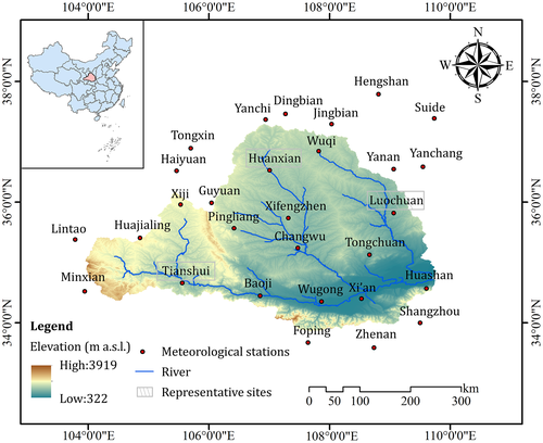
Meteorological data from 29 sites distributed within and around the study area (Figure 1) were used, covering the period 1959–2008, obtained from the China Meteorological Data Service Centre (http://loess.geodata.cn/). The average spatial density of the precipitation stations is 0.011 sites per 100 km2. The data included original variable X as annual average relative humidity (HUM), annual average maximum temperature (MAX), annual average minimum temperature (MIN), annual average wind speed (WND), and original variable Y as annual MDR at different frequencies (10%, 25%, 50%, 75%, and 90%) calculated by measured rainfall data at these observation sites. Table 1 provides a statistical summary of all selected data.
| Variable | Min | Mean | Max | STD |
|---|---|---|---|---|
| Annual maximum daily precipitation 10%(mm)—P10 | 51.34 | 77.43 | 115.55 | 13.61 |
| Annual maximum daily precipitation 25%(mm)—P25 | 42.04 | 61.00 | 89.49 | 10.59 |
| Annual maximum daily precipitation 50%(mm)—P50 | 33.53 | 46.60 | 66.88 | 8.48 |
| Annual maximum daily precipitation 75%(mm)—P75 | 25.94 | 35.87 | 51.26 | 7.07 |
| Annual maximum daily precipitation 90%(mm)—P90 | 19.93 | 28.93 | 42.50 | 6.02 |
| Annual average relative humidity—HUM | 0.50 | 0.61 | 0.71 | 0.06 |
| Annual mean maximum temperature (°C)—MAX | 8.43 | 15.47 | 19.12 | 2.53 |
| Annual mean minimum temperature (°C)—MIN | −0.10 | 4.13 | 9.23 | 2.69 |
| Annual mean wind speed (m/s) WND | 1.07 | 2.21 | 4.76 | 0.88 |
To evaluate the performance of the NLCCA-GAM model in the estimation of extreme rainfall quantiles at ungauged sites, Huanxian (HX), Luochuan (LC), and Tianshui (TS) sites with measured records were chosen as the target sites, that is the assumed ungauged sites, according to the geographical location of meteorological observation sites and the spatial distribution of precipitation. The assessment can be made by comparing estimations and observations of extreme rainfall quantiles at target sites. The locations of the target sites chosen are shown in Figure 1, with gray boxes.
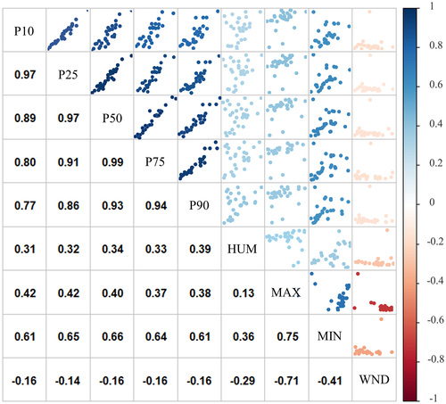
Figure 2 shows the relationship between variables. The upper-right corner shows the scatter plots of the annual MDR quantiles and meteorological variables in the Wei River basin. Examination of the scatter plots shows different forms of relationships between variables. For instance, variables P10, P25, P50, P75, and P90 show linear relationships, representing the complex nonlinear relation with variables HUM, WND, MIN, and WND. The lower-left corner of the figure presents the correlation coefficients between meteorological variables and annual MDR quantiles. It is seen from the corner that there are relatively strong positive correlations between the quantiles and MIN, and all correlation coefficients exceed 0.6. On the other hand, negative linear correlations occur between quantiles and WND, and all correlation coefficients range from −0.16 to −0.14. It can be observed from the whole scatter plot that these relationships between variables are rather nonlinear, and the nonlinearity is complex for some paired variables, such as HUM and MAX.
3 METHODOLOGY
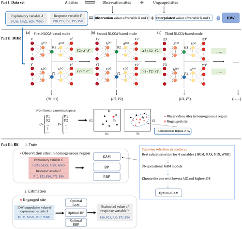
In this study, the GAM was combined with an NLCCA procedure to build the input–output model with explanatory variables (X: HUM, MAX, MIN, WND) and response variable (Y: P10, P25, P50, P75, P90). The IDW interpolation method was employed to interpolate variables X at ungauged sites from variables X measured at surrounding sites, as the input of the NLCCA-GAM model. The BP and RBF were used as the substitute for GAM to build comparative models with NLCCA-GAM. Figure 3 shows a schematic representation of the estimation of extreme rainfall quantiles at ungauged sites via RFA.
3.1 Inverse distance weighting
3.2 Delineation of homogeneous regions
Three feedforward neural networks (NNs) were used to perform NLCCA, as illustrated in Figure 3a. The double-barreled NN on the left mapped from the inputs X and Y to the canonical variates U and V. Given the variables X, the information was then mapped to the next layer—a “hidden” layer , for input Y, followed by a hidden layer . The mapping continued onto U and V. The cost function maximized the correlation between U and V. On the right side, the top NN mapped from U to a hidden layer , followed by the output layer . The bottom NN mapped from V to a hidden layer , followed by the output layer . The cost function made the mean square error between (X, Y) and (, ) minimum (Hsieh, 2000).
3.3 Regional extreme rainfall quantile estimation
3.3.1 Generalized additive model
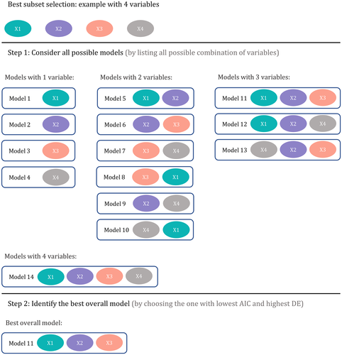
Meanwhile, a stepwise variable selection procedure (Peduzzi et al., 1980) was carried out to ensure that the optimal GAM was selected and details are shown in Figure 4. The Akaike information criterion (AIC) and deviance explained (DE) criteria were used to evaluate and compare the performances of different GAMs. In the comparison, explanatory variables (HUM, MAX, MIN, and WND) were gradually put into the comparative models with different combinations. The optimal GAM was selected according to the maximum DE principle and the minimum AIC criteria (Chebana et al., 2014).
3.3.2 Artificial neural network
The BP and RBF are two of the most recommended ANN methods worldwide, and have been successfully used in prediction with inconsistent data due to their robustness and reliability. The BP neural network, proposed by Rumelhart et al. (1986), is a standard neural network method that generally works well. It has been shown mathematically that BP has the ability to realize any complex nonlinear mapping. The hidden layer uses the global sigmoid function. Variables enter the network from the input layer, are then processed by the hidden layer, and are finally transmitted to the output layer. If the network error between the actual output and the expected output is unacceptable in the operation process, the error is used as an adjusted signal and propagated from the output layer to the hidden layer, and finally to the input layer. At this time, the weighting is adjusted to more reasonable values to reduce the network error (Al-Mahallawi et al., 2012; Rumelhart et al., 1986).
RBF model is a neural network structure proposed by J. Moody and C. Darken in 1989, which is a commonly used ANN model for function approximation problems (Moody & Darken, 1989). The RBF neural network structure contains three layers: input layer, hidden layer, and output layer. The hidden layer contains a number of nodes, which use local RBF to apply a nonlinear transformation to the input variables. The output layer is the linear summation unit. It has been shown that RBF has fast learning ability and excellent approximation performance in the fields of function approximation, pattern recognition, and signal processing (Chang & Chen, 2003; El Shafie et al., 2012).
3.4 Performance criteria
To evaluate the performance of single IDW, NLCCA-GAM, NLCCA-BP, and NLCCA-RBF models, two criteria were employed in this study:
4 RESULTS
4.1 IDW interpolation
To do the interpolation of rainfall quantiles, six to eight gauged sites were preliminarily selected as auxiliary sites serving for the estimation of quantiles at target sites according to the relative distance. Three groupings, including target and auxiliary sites, are shown in Figure 5.
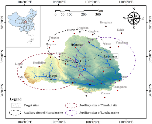
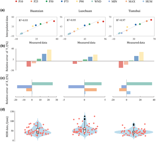
Figure 6 shows the IDW interpolation results of nine variables at the three target sites. Here, Figure 6a shows the scatter plots of observed data and the estimated values of all variables, and their correlation coefficients at the three sites all exceed 0.9. Figure 6b,c shows the relative error between the IDW interpolated values and measured data of variables Y and X, respectively. It is seen from Figure 6b that the IDW interpolation result of P50 has the lowest value (7.30%, 1.66%, 5.36%), the error of P90 being the highest (36.82%, 29.29%, 20.84%), and others have minor deviations among all variables Y. These results indicate that the IDW has a good performance in the estimation of extreme events, however, significant limitations in the severe extreme values of the MDR. It is consistent with the previous studies (Zou, Yin, & Wang, 2021b). Spatially, the interpolation errors of variable Y are lower at the TS site than at the HX site and LC sites. It may be because the range of MDR data of the TS site is smaller or MDR data are more concentrated compared with others, as shown in Figure 6d, which shows that the IDW interpolation can lead to a relatively accurate estimation in the TS site. From Figure 6c, it can be found that variables X have very low errors, and the TS site has the highest value, which is probably attributed to the long distance of the auxiliary site from the TS target site and the un-utilization of sites below the TS site.
4.2 Homogeneous regions delineation
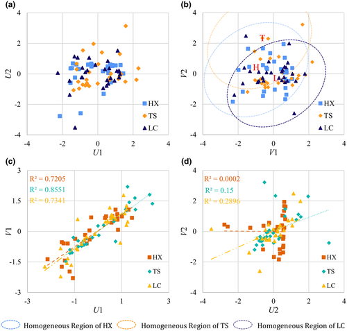
In order to determine the homogeneous region, NLCCA analysis was carried out in the DHR step. The first NLCCA-based mode obtained the first pair of canonical variables (U1, V1). The second NLCCA-based mode got the second pair of canonical variables (U2, V2). Figure 7 presents the scatter plot of U1, V1, U2, and V2 in the nonlinear canonical spaces at three study sites. Therein, (U1, U2) refers to the explanatory variables, as shown in Figure 7a, and (V1, V2) refers to MDR quantiles, as shown in Figure 7b, (U1, V1) refers to the first pair of canonical variables, as shown in Figure 7c, and (U2, V2) refers to the second pair of canonical variables, as shown in Figure 7d. Additionally, the DHR results of HX, TS, and LC calculated by NLCCA are shown in Figure 7b. In the last two subgraphs, a strong positive linear correlation of the canonical variables (U1, V1) and a very weak linear relationship of the canonical variables (U2, V2) are seen through the R2 values. It implies that a lot of important information between the original explanatory and response variables has been extracted, and more modes are not required.
4.3 Building GAMs
The GAM was constructed using the “mgcv” package (https://CRAN.R-project.org/package=mgcv) in the R language and environment. In RE step, explanatory variable X and response variable Y of measured sites in the homogeneous region of a target site were employed as the training data of GAM. Also, a stepwise variable selection procedure was used to get optimal GAM at the target site. Figure 8 shows the selection process of the optimal GAM for response variable P10. Here, 36 operational GAMs were established according to a stepwise selection procedure. The AIC and DE values were employed as the evaluation criteria to 36 models, and results are shown in Figure 8a. It was found from model calculations that the crashes occurred in this program running, showing the abysmal performance of the model when variables HUM, MAX, MIN, and WND were input together in the selection process. However, the stepwise method for the variable selection solved this issue, implying the advantage in improving the quantile estimation. Depending on the evaluation results of 36 models, the model with the variables HUM, MAX, MIN, and Gamma distribution was chosen for P10 due to the low AIC value and the high DE value of this model (HUM-MAX-MIN). Also, this model is appropriate for other response variables, that is, P25, P50, P75, P90.
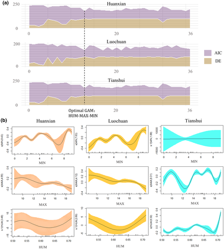
As is well known, the GAM is a tool to identify the effect of each explanatory variable on the corresponding response variable, and can represent the nonlinear and complex relationship between response and explanatory variables through smooth functions. Figure 8b illustrates the relationship of the explanatory variables (e.g. HUM) with the smooth functions (e.g. s(HUM, 8.39)) of the response variable P10 at the three target sites, in which the degree of freedom (e.g. 8.39) in the title of vertical coordinate can effectively reveal the nonlinear relationship between the explanatory variables and P10. In this figure, all the estimated degrees of freedom of s(HUM), s(MAX), and s(MIN) are much larger than 1, implying P10 has a strong nonlinear relationship with variable X. To other response variable Y, the similar nonlinear relationships were also seen. It indicates that the GAM is more flexible in describing the relationship between response and explanatory variable, with the advantage not only in linearity but also in nonlinearity.
To compare among different models, the same variable data were used to train the BP and RBF models, and then the optimal structures of the two models were obtained.
4.4 Estimation of extreme rainfall quantiles
The IDW interpolation data of variable X at target sites were taken as the input values of the optimal GAM, BP, and RBF model, and the response variable Y can be estimated at these sites. The relative error of the NLCCA-GAM model is illustrated in Figure 9a. Here, the maximum error (12.69%) appears in the estimation of P10 at the TS site, and the minimum error (0.28%) is in that of P75 at the LC site. The relative error of the NLCCA-BP model is illustrated in Figure 9b. The maximum error (50.04%) appears in the prediction of P10 at the TS site. The minimum error (4.48%) appears in the prediction of P25 at the HX site. From this, it can be found that the BP model might be poorly estimated at the TS site compared with other sites. The relative error of the NLCCA-RBF model is illustrated in Figure 9c. The maximum error (51.06%) appears in the prediction of P10 at the TS site. The minimum error (8.84%) appears in the prediction of P50 at the TS site. The RBF model achieves a good estimation performance at the HX site compared with other sites. Also, the performance of the NLCCA-RBF approach for variables Y has significantly varied.
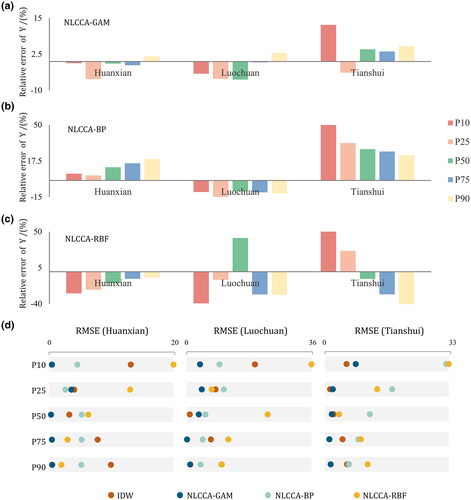
Figure 9d shows the RMSE results of all considered models at the three target sites. In the analysis of all RMSE values, the best results of the single IDW, NLCCA-GAM, NLCCA-BP, and NLCCA-RBF models among all data were 0.91, 0.12, 2.58, and 1.94, respectively, and the worst results were 19.53, 8.07, 31.81, and 35.71 for P10.
At the HX site, the RMSE values for the single IDW were in the range of 3.20–13.00. The RMSE values were in the range of 0.31–3.53 for NLCCA-GAM, and were in the range of 2.58–5.19 and 1.94–19.78 for the NLCCA-BP and NLCCA-RBF, respectively. In terms of overall performance, NLCCA-GAM > NLCCA-BP > IDW > NLCCA-RBF for the HX site.
At the LC site, the RMSE values were in the range of 0.91–19.53, 0.12–4.32, 3.96–10.63, and 7.15–35.71 for the single IDW, NLCCA-GAM, NLCCA-BP, and NLCCA-RBF, respectively. The overall performance at the LC site was ranked from the highest to the lowest as follows: NLCCA-GAM > NLCCA-BP > IDW > NLCCA-RBF.
At the TS site, the IDW and NLCCA-GAM models had the RMSE values ranging from 1.31–5.78, and 1.15–8.07, respectively. The NLCCA-BP and NLCCA-RBF models had the RMSE values ranging from 6.26–31.81, and 3.69–32.46, respectively. On the whole, NLCCA-GAM > IDW > NLCCA-BP > NLCCA-RBF in estimation performance, as shown in Figure 9d. However, the estimation performance of the NLCCA-GAM, NLCCA-BP, and NLCCA-RBF was poor at the TS site. This may be attributed to the interpolated result of variable X at the TS site with a high error.
To sum up, it can be concluded that the NLCCA-GAM model produced better results than other comparative models, followed by the NLCCA-BP approach, implying the hybrid model (NLCCA-GAM) combining the NLCCA with GAM had an advantage in the estimation of extreme rainfall quantiles.
5 DISCUSSION
In the sections above, the MDR quantiles at the three sites were estimated. Here, to evaluate the performance of single IDW, NLCCA-GAM, NLCCA-BP, and NLCCA-RBF models in the estimation of the MDR quantiles in the whole study area, all considered models and more target sites (Xi'an, Changwu, Pingliang, Tongchuan, Xifengzhen, and Xiji sites) were employed. Figure 10a summarizes the estimation performance of all models for variable Y at all target sites. Results indicated that the NLCCA-GAM approach significantly outperformed other approaches in terms of RMSE. Specifically, the best results (low RMSE) of P10, P25, P50, P75, and P90 were all associated with the NLCCA-GAM. There, the estimated values of P10 had bigger RMSE than P25, P50, P75, and P90, but far less than the error of other models. Among all models, the single IDW and NLCCA-GAM models showed better performance in the estimation of P25 and P50, and the smallest RMSE values of P10, P75, and P90 were associated with NLCCA-GAM and NLCCA-BP. For the estimation of P75 and P90, the hybrid approaches (NLCCA-GAM, NLCCA-BP, and NLCCA-RBF) using nonlinear tools in both RFA steps outperformed the linear approach (single IDW). In addition, compared with the IDW model, the RMSE values of NLCCA-GAM for P10, P25, P50, P75, and P90 were reduced by 71%, 55%, 61%, 63%, and 78%, respectively. Compared with the NLCCA-BP model, the RMSE values reduced by 70%, 72%, 64%, 53%, and 67%. Compared with the NLCCA-RBF model, the corresponding values reduces by 84%, 76%, 79%, 60%, and 71%. Figure 10b compares the results of two better full nonlinear models (NLCCA-GAM and NLCCA-BP) mentioned above at all 29 sites in the Wei River basin. The horizontal axis represents the observed data and the vertical axis represents the estimated values. It can be seen from the figure that the correlation of values estimated by NLCCA-GAM with the measured data is superior to that of NLCCA-BP in the whole basin through coefficient R2, which also supports the conclusion mentioned in Section 4.4 that the NLCCA-GAM has the best performance in the estimation of extreme rainfall quantiles.
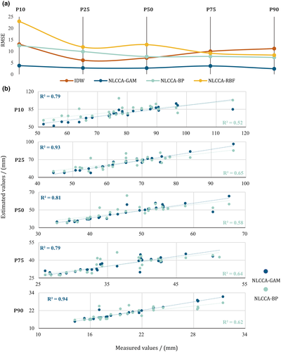
Through the above analysis, the good estimation performance of the NLCCA-GAM model can be attributed to two aspects. The first is the combination of the advantages of the nonlinear delineation method and the generalization ability of the nonlinear regional extreme rainfall quantile estimation method. As is well known, the advantages of IDW refer to the intuition and efficiency in interpolation, but its interpolation performance generally depends on the distribution uniformity of sites with observed data. The IDW could work well at a very low efficiency if the measured sites are uneven. What is more, studies indicate that IDW is not satisfactory in estimating severe extreme events. The NLCCA-GAM can do the estimation based on the results of DHR, not bound by the distribution uniformity of sites. The other one is that GAM outperforms BP and RBF when combined with the same NLCCA delineation method. The reason is considered that the training dataset is not too large in the Wei River Basin, causing the ANN models to be poorly trained and further cannot work fully effectively. However, the GAM has advantages in explaining the relation between response and explanatory variables, and overcoming the impact of excessive explanatory variables. Thus, NLCCA-GAM provided the most accurate estimations compared to all other approaches in this study. To sum up, the NLCCA-GAM has stronger robustness in estimating quantiles of annual MDR. Meanwhile, a nonlinear relationship does exist between hydro-meteorological variables in the Loess Plateau, China.
6 CONCLUSIONS
The main objective of this study is to investigate the applicability of NLCCA-GAM-based RFA to estimate MDR quantiles in Loess Plateau, China. In the investigation, temperature, HUM, and WND are employed as explanatory /input variables, and MDR at different frequencies is used as response/output variables. IDW is applied to interpolate explanatory variables at ungauged sites. Three comparative methods including single IDW interpolation, NLCCA-BP, and NLCCA-RBF are introduced for testing the efficiency of the NLCCA-GAM model.
The interpolation results reveal that IDW has a good performance in the estimation of extreme events, and obvious limitations in severe extreme values of the MDR, representing the significant under-estimation for P10, and remarkable over-estimation for P90.
Comparative results among various models indicate all models perform “poorly” in the estimation for P10. Fully nonlinear models (NLCCA-GAM, NLCCA-BP, and NLCCA-RBF) have the best estimation performance for P90. The single IDW interpolation and NLCCA-GAM models work well for P25 and P50. The errors of NLCCA-GAM and NLCCA-BP models are significantly lower than others for P10, P75, and P90. On the whole, the NLCCA-GAM approach significantly outperforms the NLCCA-BP, NLCCA-RBF, and single IDW approaches, with the lowest relative error and RMSE.
Performance analysis shows that the NLCCA approach provides a flexible delineation of homogeneous neighborhoods, and is not enslaved to distribution uniformity of the sites with observed data. The GAM approach has an advantage in adequately accounting for the nonlinearities between hydro-meteorological variables. The combination of IDW (interpolation), NLCCA (DHR), and GAM (RE), namely a hybrid model of IDW-NLCCA-GAM is a valuable tool for the estimation of extreme rainfall quantiles.
As is well known, the general lack of hydro-meteorological data in many regions worldwide often makes it difficult to establish accurate hydrological models for flood control, water resources assessment, river basin management, and hydrological forecasting in the data-scare areas. As a result, the estimation of hydro-meteorological variable quantiles at ungauged sites should be given more attention, and the IDW-NLCCA-GAM hybrid model may be considered in more fields.
Some issues should be noted in the application of the proposed model. The first one is the sample size. As well known, GAM as well as ANN models, require much data for the calibration and validation of the model. Therefore, a sufficient sample is necessary to obtain the expected performance. The second is the identification of optimum parameters and the selection of the transfer function in NLCCA, which require some practical experience in model parameter adjusting. The last and most important one is the selection of explanatory variables. Due to the hydrological system being usually highly nonlinear and complex, excessive explanatory variables tend to be considered for the response variable. However, it is not necessarily appropriate because it may bring a huge amount of work in building GAMs. In addition, it may be of interest to proceed with other statistical techniques such as CCA or MLR for the estimation of rainfall quantiles.
ACKNOWLEDGMENTS
This study was supported by the National Natural Science Foundation of China (51979005 and 51809005) and the Natural Science Basic Research Program of Shaanxi (2020JM-250).
CONFLICT OF INTEREST
The authors declare no conflict of interest.
Open Research
DATA AVAILABILITY STATEMENT
Meteorological data from 29 sites in study area was obtained from the China Meteorological Data Service Centre (http://loess.geodata.cn/).


