2.1 Structure locations, characteristics, and value

We base our analysis on a publicly available digital parcel map for 2,340,303 tax parcels in Massachusetts (MassGIS, 2019), excluding Suffolk County (the City of Boston), for which we use a commercial digital map of 127,203 tax parcels, provided by Regrid. Parcels are linked to the ZTRAX nationwide tax assessor and transaction database (Zillow, 2021), as well as a dataset for flood hazards open to researchers (First Street Foundation, 2020) and other open-source datasets (for details, see, Table S2). These inputs were harmonized to the parcel level using the Private-Land Conservation Evidence System (PLACES) database (Nolte, 2020) to yield our dataset of 1.3 million single family homes.

Following Nolte et al. (2021), we identify residential buildings as those with corresponding ZTRAX building codes (RR101, RR102, RR000, and RR999) and at most two building footprints linked to a parcel. Remotely sensed building footprint data can omit buildings that are under tree cover or newly constructed. We include properties without building footprints if a building valuation is recorded by the tax assessor and assume that the building is located at the centroid of the parcel. Properties with more than two building footprints are assumed to exhibit too much uncertainty in structures' locations. Building geocodes are used to identify whether a property is in a FEMA flood zone and for linking properties to high-resolution flood hazard datasets (Section 2.2, below).

Accurate calculation of losses necessitates information on the values and characteristics of flood-affected structures, a variable which tends to be unreported or heuristic and unvalidated (for details, see, Supporting Information). For properties with recorded sales, we impute the structure value by multiplying each property's deflated ZTRAX sale price (FHFA, 2020) by the ratio of the assessed value of the building to the assessed value of the property (i.e., building and land). Where sales data are missing, the assessed value of the building is used. Assignment of characteristics to structures is based on architectural characteristics recorded in ZTRAX. For the remainder, we use the universe of OpenFEMA NFIP Redacted Policies dataset to define spatially varying probabilities of structure (FEMA, 2019), similar to the approach in Aerts et al. (2014). (For details, see, Supporting Information).

2.2 Flood hazards

Our flood hazard estimates are based on 30 m horizontal resolution modeled spatial distributions of inundation depths on 2, 5, 10, 50, 75, 100, 200, 250, and 500 years return periods, developed by First Street Foundation (2020). These incorporate fluvial and pluvial processes inland (Wing et al., 2017), and fluvial, pluvial, and coastal processes within 100 km from coastlines (Mandli & Dawson, 2014). In areas with no surge or tidal hazard, the model selects the maximum of fluvial and pluvial depth. A one-dimensional hydraulic model is used to capture fluvial processes (Bates et al., 2021), distinct from two-dimensional (2D) approaches employed to generate recent flood insurance rate maps (FIRMs; FEMA, 2020a), and with further potential differences in stream geometry (Bates et al., 2021; Benjankar et al., 2015; FEMA, 2020a). In coastal zones, surge, fluvial and pluvial hazards are modeled individually and then jointly to identify joint effects of each source of hazard on flooding (First Street Foundation, 2020). We use the 2020 mid-likelihood depth and link the flood hazard estimates to our parcel data using spatial joins of the lowest point of a building footprint or, where no footprint is available, the parcel centroid.

2.3 Depth-damage functions and property-level inundation exposures

We utilize physical depth-damage functions (DDFs) that specify fractional loss in the value of a structure resulting from different flood depth exposures. Our DDFs are taken from the US Army Corps of Engineers' (USACE) North Atlantic Coast Comprehensive Study–NACCS (USACE, 2015). In contrast to the more widely used HAZUS-MH functions (FEMA, 2021b), NACCS DDFs specify “minimum,” “most likely,” and “maximum” damage curves for different building archetypes. NACCS DDFs are further stratified according to building archetypes whose characteristics determine vulnerability to inundation: the type of foundation (including the presence of a basement), the height of the FFE, and the age of the structure. (See, Table S3). Each home in our sample is assigned to an archetype, based on the presence of a basement, the number of stories, and the structure's age. We calculate damage using DDFs for one-story and two or more story single-family residences, with and without basements (Figure S1). Where the basement and/or number of stories are unknown, we calculate losses using damage curves for every archetype, weighting the outcome by the fraction of houses corresponding to each archetype in the property's flood zone, tract, or county, similar to Aerts et al. (2014). (For details, see, Supporting Information).

A crucial uncertainty is that nonzero depth above grade at the building centroid may or may not translate into damage. The literature contains scant guidance on how to deal with such situations (FEMA, 2021b; USACE, 2015). Our approach is to subtract the archetypical value of the FFE assigned to each building from the depth given by the hazard layer to obtain an “effective depth” that is used as input to the appropriate DDF for that building. For basement homes in particular, damages can occur at negative depths relative to grade. To assess the sensitivity of losses to our algorithm, we augment our default model (“Benchmark”) with illustrative alternative specifications (“Damage Scenarios”) that illustrate the impact of FFE adjustments and the choice of damage curves (“minimum,” “most likely,” or “maximum”) within each building archetype (Table S3).

2.4 Loss estimation: the benchmark procedure

2.5 Aggregation procedures and bias quantification

2.6 Aggregation bias metrics and drivers

It is extremely challenging to predict the a priori net impact that each of our procedures could have on EAL—either in aggregate, or in terms of the distribution of losses across spatial units. First, Equations (1a), (3a), (4a), and (5a) highlight that losses increase linearly with the value of affected assets. The fact that distributions of building values tend to be long-tailed (Tate et al., 2015) suggests that upper tail property values will account for a large proportion of losses (Kousky & Walls, 2014; Tate et al., 2016). To the extent that, all three aggregation procedures underestimate these tail values the resulting EAL bias would be negative.

Second, this seemingly straightforward effect is complicated by the influence of fine spatial scale topographic heterogeneity. On one hand, naïve aggregation of flood hazards that ignores the possibility that some properties have zero depth exposure will erroneously apply damage to valuable structures that are in fact undamaged, biasing aggregate EAL upward. But on the other hand, the calculation of the aggregated hazard will include these zero-depth observations, imparting a downward bias to aggregated depths, and, for damaged properties, percentage losses, leading to underestimation of EAL. The degree to which the error in one or the other direction dominates, or the two fortuitously cancel out (Merz et al., 2010), depends on the relative numbers of properties that are undamaged and erroneously identified as exposed versus those truly at risk, the distribution of depths faced by the latter (which are likely to also exhibit long tails—(Tate et al., 2015)), and the convexity of the damage function.

Third, further complications arise from the potential for aggregation to alter DDFs' shapes and change the relationship between DDFs and structure values. Aggregating over structures can lead to biases in the assignment and/or weighting of structural archetypes—and their damage susceptibility (Figure S2). The direction of this effect is highly uncertain. Moreover, structural characteristics and values are likely both highly correlated with one another, and jointly correlated with depth exposure (Beltrán et al., 2018; Pollack & Kaufmann, 2022). To the extent that aggregation procedures fail to preserve such correlations, they may underestimate EAL by failing to capture high-value homes that incur substantial damage from extreme depth exposures on long return periods.

The ultimate goal is to rigorously evaluate the importance of these factors in the context of global sensitivity approaches of the kind used by Tate et al. (2015). However, given the complexity and computational cost of undertaking such an analysis with large-scale data, we settle here for the more modest interim step of elucidating the potential pitfalls of input aggregation that capture in a stylized way the essence of procedures commonly seen in practice.

To quantify the overall severity of bias we compute summary statistics of the fine-scale agreement between aggregated and benchmark EAL: the root mean square error (RMSE), a common accuracy metric, which is strictly positive, and bias per home at risk, an accuracy metric which also indicates the direction of estimation error. To quantify the impact of aggregation on the distribution of EAL, we calculate the agreement in the rank ordering of losses via the standard error of rank order bias (see below, Equation 8). All three metrics are computed at the property level and for loss aggregated to the census tract, the finest scale at which analyses utilizing aggregation procedures cited in Table S1 present their results. We also compute our metrics at the county level, to test whether bias cancels out over larger units of aggregation.

We also elucidate the potential drivers of bias. First, we inspect the spatial patterns of depth and structure value for aggregation-based procedures compared to the benchmark. We then capture the overall influence of the shape of the input distributions by computing how the joint and marginal densities of depth and building value under each procedure shift with respect the benchmark. Finally, we demonstrate how aggregation-induced errors in the number of properties at risk, property value, and the damage function interact with uncertainty in the structural archetypes—particularly in the tails of the distributions of depth and value.

3.1 Total aggregation bias and its spatial distribution

We find that all data aggregation procedures introduce biases in the estimation of expected annual flood losses (Figure 1). Our benchmark derived from all high-resolution data (hazard and structures) estimates that 139,836 single family homes in Massachusetts are exposed to flood risk, giving rise to a total EAL of $374 million (Figure 1, Table S4). Relative to this benchmark, aggregating structures to the block group (AS) underestimates total EAL by 17% (Figure 1a); it also leads to a slight overestimation of the number of properties at risk (+1%) (Figure 1b), mainly due to differences in the applied DDFs and the resulting extent to which structures are estimated to incur losses at low depth. By contrast, additionally aggregating hazard to the census block without removing not-at-risk properties (ASH) leads to a substantial overestimation of the number of properties estimated to be at risk (by a factor of 4.5) as well as total EAL (by a factor of 3.7; Figure 1a,b). When properties not at risk are removed prior to aggregation of structures and hazard (ASHF), this bias in total EAL is reduced to +44% relative to the benchmark (Figure 1a), a substantial reduction when compared to the ASH procedure, but still a large overestimate.

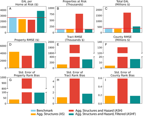
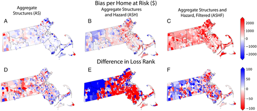
None of the aggregation procedures succeed in accurately capturing the distribution of expected flood losses across Massachusetts single-family homes (Figures 1 and 2). At the property level, RMSE exceeds benchmark EAL per home at risk regardless of procedure (Figure 1a,d) and procedures based off aggregate inputs generally fail to capture the rank ordering of losses (Figure 1g). At the level of census tracts, we observe the largest biases—a RMSE and standard error of rank order bias of $1,948,066 and 4.5, respectively—when aggregating both structure and hazards without removing not-at-risk properties (ASH) (Figure 1e,h). Tract-level bias is reduced by a factor of over 6 to an RMSE of $308,668 and a rank order discrepancy of 1.8 when properties not at risk are removed (ASHF). Aggregating structures only (AS) leads to the lowest errors in spatial distribution: a RMSE and standard error of rank order bias of $129,016 and 1.1, respectively. However, even in this latter case, biases for individual census tracts can be large. Furthermore, over- and underestimations are clustered in space (Figure 2). These biases and errors in rank ordering persist even when loss estimates are aggregated to coarser spatial units, such as the census tract or county (Figures 1, 2, and S5), illustrating that errors observed at small spatial scales do not necessarily cancel out when aggregating to larger spatial scales.

3.2 Aggregation fails to capture joint long-tailed distributions of hazard and structure value

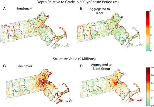
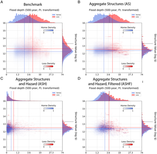
A key driver of the observed aggregation biases is the joint distribution of estimated flood hazard (depth) and structure values. In Massachusetts, these distributions are both positively skewed, and the long upper tails are spatially correlated with each other. For example, many of the highest-value homes are clustered along much of the coast, which coincide with locations facing relatively high depths (Figure 3a,c). This correlation of high-value and high-hazard homes drives results in overall loss estimation as illustrated by 8.5% of total EAL in the benchmark procedure composed of only 0.6% of properties that are in the top 10% percentiles of both value and hazard distributions. This crucial interaction is largely lost when input data is aggregated along either dimension (Figure 4). The joint distributions of all observations versus loss-weighted observations (Figure 4a) are substantially reduced through aggregation of structures (Figure 4b–d) and hazard (Figure 4c,d). Importantly, average flood depths in the ASH procedure are considerably lower than in other procedures since they include homes not at-risk within each block. Adjusting for this overinclusion with a filter for homes at-risk (ASHF) improves the representation of average depth, but the misrepresented marginal and joint distributions still lead to substantial bias (Figures 1c, 2c, and 4d). Finally, the AS procedure generates marginal distributions for structure value based off all observations and loss-weighted observations that is narrower than under the high-resolution benchmark. As a result, even though average structure value is roughly captured, the joint distributions in the upper tails of depth and structure value are not, with a greater density of observations closer to the means of depth and structure value. This explains the overall underestimation of losses from this procedure (Figure 1c), and prominent underestimations of loss in high-valued coastal areas (Figure 2a).

3.3 Aggregation of structure characteristics can introduce additional bidirectional biases

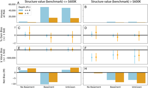
In addition to the observed loss of long-tailed distributions through aggregation, we observe that the aggregation of structural characteristics can introduce additional over and underestimations of loss, because the convexity of DDFs varies by structure type and depth. This rather complex relationship can be illustrated by decomposing overall bias in our best-performing aggregation procedure—the aggregation of structures (AS)—by depth, value, and a key structural characteristic, namely whether a home has a basement (Figure 5). We find that bias in the estimation of fractional damage (i.e., % of structure value) increases with estimated hazard (flood depth), as does the standard deviation of estimation errors (Figure 5c,d). These biases are bidirectional: on average, percentage damage is underestimated for homes with basements and overestimated for homes without basements or no (i.e., imputed) basement information; this is the case both for the tail of highest-value structures (>$600K) as well as the remainder. However, because estimated fractional damage interacts (i.e., is multiplied) with bias in structure value (Figure 5e,f) and the total number of properties (Figure 5a,b), overall bias in the EAL estimation varies among subgroups in directions other than one might assume when considering only the observed biases in the estimation of fractional damage. For instance, although homes with unknown basement type have a negative average bias in fractional damage, their estimated EAL is overestimated on net when highest-value structures are excluded (Figure 5g). Conversely, in the case of highest-value structures, the large negative bias in the aggregation of structure value prevails over the bias in fractional damage (Figure 5f), leading to an underestimate of EALs across all structure types. This illustration highlights that interactions between flood hazard, structure characteristics, and structure value can give rise to net biases that can be difficult to predict and correct for ex-ante when an analyst only has access to aggregated data. Importantly, the relationships observed in the case of Massachusetts might look different in other locations.

3.4 Benchmark losses are highly uncertain

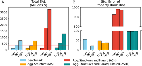
Finally, we find that estimates of EAL can be highly sensitive to key assumptions analysts have to make with respect to unobserved structural characteristics, notably the FFE of homes relative to grade and the shape of DDFs. Differences between benchmark estimates based on “low damage,” “reference,” and “high damage” assumptions are an order of magnitude larger than biases introduced through the aggregation of structures (AS) or through the aggregation of structures and hazards when properties not at risk are removed (ASHF) (Figure 6). Similarly, differences in the distribution of property-level EAL estimates are of similar magnitude as those introduced through data aggregation (Figure 6).

4.1 Accurate flood loss estimation requires high-resolution data on hazards and structures

Our results reveal the potential for substantial aggregation bias in the estimation of flood loss when input data on hazard and structures are aggregated to even relatively small spatial units (census blocks). This threat appears to be particularly high if the distributions of flood hazard and structural value are positively skewed and their tails are correlated in space. Due to complex interactions between flood hazards, structure values, and structure characteristics, there is no easy remedy to control for this bias when high-resolution data is not available for large-scale estimation tasks.

These findings have important implications for applications that rely on the estimation of flood risk over large scales, like calculating flood insurance premiums. For instance, we find that the aggregation of data on structures (AS)—with which we sought to emulate the aggregation procedures inherent in RR 2.0—underestimates total EAL by 17% in our case study. Although this bias is smaller than those introduced through the aggregation of flood hazard (ASH and ASHF), or through potentially erroneous imputation of key missing data, such as FFE, it could negatively affect the solvency of an insurance scheme that relied on this strategy for the computation of premiums.

Similarly, our results demonstrate that flood loss estimation procedures that rely on aggregate input data will find it challenging to accurately reproduce the spatial distribution of flood risks across individual properties and broader spatial scales (Figures 1, 2, and S5). As a result, such procedures are unlikely to be suitable for the identification of actuarially fair flood insurance premiums (RR 2.0), or for the efficient allocation of flood mitigation funding to different communities (Johnson et al., 2020; Narayan et al., 2017; Reguero et al., 2018). In the case of the NRI, the reliance on flood zone boundaries to identify properties at risk, and their exposure, likely introduces additional substantial errors in terms of overall bias and rank ordering of units at risk because flood zones include homes not at risk, exclude homes at risk, and do not capture fine-scaled heterogeneities of exposure and vulnerability (Czajkowski et al., 2013; Wing et al., 2018; Figure S6). However, an underlying issue we do not address is the differences between the hydraulic modeling approaches employed by the First Street Foundation and FEMA, and their potentially divergent effects on inundation depths and extents—a question that is a key area for future research. More generally, high-resolution estimation of flood losses draws attention to situations in which the majority of flood losses, and thus the majority of benefits of flood mitigation, are likely captured by the highest-value homes, thus shedding light on potential equity issues in the allocation of federal and state funding if based on procedures subject to aggregation bias.

4.2 Missing data is a substantial source of potential bias that remains largely unmitigated

In addition to the issue of aggregation bias, our results draw attention to key uncertainties in the estimation of expected flood losses that cannot be easily resolved using the property-level datasets commonly available to flood researchers (e.g., tax assessor data). Although joint observation of building footprints and terrain elevation is now feasible and continuously improving (Hawker et al., 2022), missing data on other key characteristics—such as FFE and the presence of basements—remains a major source of uncertainty and potential bias in the estimation of flood losses (Figure 6). To shed further light on the relative importance of different data imputation assumptions, flood loss estimation analyses and products need to acknowledge more fully, and attempt to model, these sources of biases and uncertainties inherent in estimation strategies, including relevant uncertainties in the underlying flood hazard model (Tate et al., 2015). Crucially, uncertainty analyses need to explicitly account for the possibility that errors in data imputation can be correlated in space (Saint-Geours et al., 2015; Tate et al., 2015). Similar error correlations can also be introduced through assumptions inherent in estimation procedures that rely on the depth-damage paradigm. For example, the linear relationship between damage and structure value could easily be violated if owners of high-value homes are more likely to invest in structural defenses to reduce flood losses, or if defended homes command a premium in the market from knowledgeable buyers (Pollack & Kaufmann, 2022). Following the logic of Equation (1a), this effect would make the damage function systematically less convex for the highest value properties, leading to an overstatement of aggregation bias at the highest depths and structure values. A dearth of systematically available property-level information on structural defenses makes it difficult to test these assumptions explicitly.

More rigorous empirical assessments of observable relationships between modeled flood depths, actual flood inundations and observed flood damages across different realized flood events and heterogeneous structure inventories could assist with the development of empirical DDFs and best-practices for prospective loss estimation (Rözer et al., 2019; Schröter et al., 2014; Wing et al., 2020). Our uniform perturbation of FFE and its effect on depth-damage relationships is a crude first step toward characterization of the relevant uncertainties. The fundamental challenges are to, first, understand how such relationships might be distributed among different property types and locations at high resolution, and second, assess the aggregate consequences of hundreds of thousands of property-level perturbations in a computationally efficient manner. With large-scale datasets of the kind used here, such an undertaking is at the forefront of uncertainty quantification research (Tate et al., 2015; Wing et al., 2022).