Relationship between the Virtual Dynamic Thinning Line and the Self-Thinning Boundary Line in Simulated Plant Populations
Supported by the National Natural Science Foundation of China (30270243).
Abstract
The self-thinning rule defines a straight upper boundary line on log-log scales for all possible combinations of mean individual biomass and density in plant populations. Recently, the traditional slope of the upper boundary line, −3/2, has been challenged by −4/3 which is deduced from some new mechanical theories, like the metabolic theory. More experimental or field studies should be carried out to identify the more accurate self-thinning exponent. But it's hard to obtain the accurate self-thinning exponent by fitting to data points directly because of the intrinsic problem of subjectivity in data selection. The virtual dynamic thinning line is derived from the competition-density (C-D) effect as the initial density tends to be positive infinity, avoiding the data selection process. The purpose of this study was to study the relationship between the virtual dynamic thinning line and the upper boundary line in simulated plant stands. Our research showed that the upper boundary line and the virtual dynamic thinning line were both straight lines on log-log scales. The slopes were almost the same value with only a very little difference of 0.059, and the intercept of the upper boundary line was a little larger than that of the virtual dynamic thinning line. As initial size and spatial distribution patterns became more uniform, the virtual dynamic thinning line was more similar to the upper boundary line. This implies that, given appropriate parameters, the virtual dynamic thinning line may be used as the upper boundary line in simulated plant stands.
 (1)
(1) (2)
(2) (3)
(3)In this paper we investigate the relationship between the virtual dynamic thinning line and the self-thinning upper boundary line in simulated even-aged plant populations. First, a spatially explicit, individual-based plant competition model based on empirical equations was developed; then the model was validated according to simulation results; finally the possibility of use of the virtual dynamic thinning line as the boundary line was discussed.
 (4)
(4) (5)
(5) (6)
(6) (7)
(7) (8)
(8)
 (9)
(9) (10)
(10) (11)
(11) (12)
(12)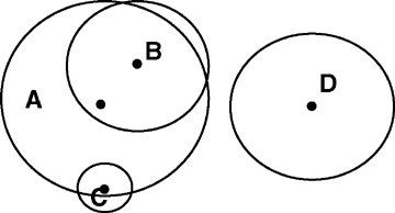
Diagram of the area of suppression (AOS) concept.White circles represent AOSs of plants, the central solid points in white circles are the original positions of corresponding plants, and the capital letters denote plants or their AOSs. In the AOS model, if the original position of plant X is in the AOS of plant Y, plant Y will suppress the growth of plant X. We say plant X is in the AOS of plant Y, and X and Y are called the suppressed plant and the suppressor plant, respectively. The intensity of suppression influence placed on plant X by plant Y is determined by their relative sizes and distance. In this diagram, plant A is a suppressor of plants B and C, but is only suppressed by plant B; plants B and A are mutual suppressors; plant C is suppressed by plant A, but is not a suppressor of plant A; plant D is isolated, and its existence and growth don't influence and aren't influenced by other plants. This diagram illustrates that neighboring individuals are not always mutually suppressing in the AOS model.
 (13)
(13) (14)
(14) (15)
(15) (16)
(16)The AOS model is an improved neighborhood model. In traditional neighborhood models (Pacala and Silander 1985; Pacala 1986, 1987; Zhang et al. 1989; Mabvurira and Miina 2002), the radius of neighborhood is fixed throughout the ontogeny of a plant. Whether two plants are neighbors is only determined by their proximity, and plants are called neighbors mutually. In the AOS model, however, AOS of a plant increases with growth of the plant, reflecting the increasing demand for more resources as plants grow larger, and plants are not necessarily neighbors mutually. Another difference between the AOS model and traditional neighborhood models is that the “neighborhood” (AOS) is defined from the point of the suppressor in the AOS model but from the point of the suppressed individual in traditional neighborhood models. When plants compete for sunlight, larger plants shade smaller neighbors and intercept more solar radiation, whereas smaller plants cannot determine which plants will shade them. So, competition for light can be studied in a more natural way by defining the AOS of a suppressor other than the neighborhood of a suppressed plant.
Results
The C-D effect
 (17)
(17) (18)
(18)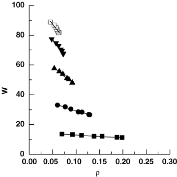
The competition-density (C-D) effect between mean plant biomass w and plant density ρ at given times.40 years(▪); 50 years ( •); 60 years(▴); 70 years(▾); 80 years (□). The curves are fitted using Equation 17.
Reciprocals of At and B in Equation 17 mean, respectively, the asymptote of yield (=wρ) and the asymptote of mean individual biomass at a given point in time. B should decrease monotonically during the development of populations. In the present runs of our model, B increased after 80 years, so only data until 80 years were used in analyzing the C-D effect. At gradually decreased from 0.321 m2/kg to 0.055 m2/kg with physical time t, while B decreased more abruptly from 5.216 kg−1 to 0.009 kg−1, close to zero (Figure 3).
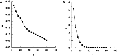
Changes of At and B in Equation 17 with physical time t.
 (19)
(19) (20)
(20) (21)
(21)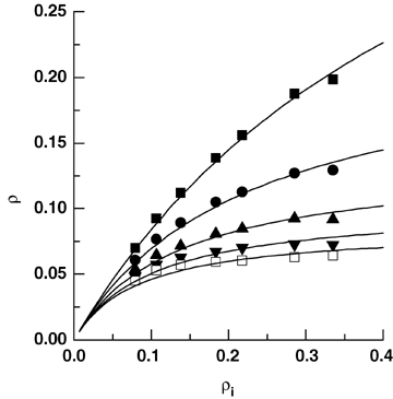
Relationship between realized density ρ and initial density ρi at given times.40 years (▪); 50 years ( •); 60 years (▴); 70 years (▾); 80 years (□). The curves are fitted using Equation 19.
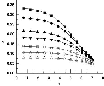
Survival curves relating realized density ρ to biological time τ in the seven populations with different initial densities.Initial plants number: 29 785 plants (▪); 25 950 plants ( •); 20 064 plants (▴); 16 560 plants (▾); 12 932 plants (□); 9 078 plants (○); 7 360 plants (□). The curves are fitted using Equation 21, with P = 0.015 m2 and μ = 0.929.
Dynamic thinning lines
 (22)
(22) , Equation 22 is rewritten as:
 (23)
(23)In the seven populations with normal initial size and random spatial pattern, the time-trajectories of combinations of mean plant biomass and plant density were seven curves concave down (Figure 6). Mean plant biomass increased as density-dependent mortality occurred, and the combinations of mean plant biomass and density eventually approached a common asymptotic line. This implicitly indicates the existence of an upper boundary line, and also illustrates the difference between dynamic thinning lines and the upper boundary line. The fitting of Equation 23 to data from the population with 29 785 initial individuals is illustrated in Figure 7, which indicates that the dynamic thinning line is well described with Ogawa's model. The values of k and −β in Equation 23 resulting from the fitting in Figure 7 are listed in Table 2.
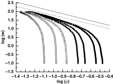
Different types of self-thinning line.The seven curves concave down are dynamic thinning lines in seven populations with different initial densities. Mean plant biomass w and plant density ρ are logarithmic transformed base 10. Initial plants number: 29 785 plants (▪); 25 950 plants ( •); 20 064 plants (▴); 16 560 plants (▾); 12 932 plants (□); 9 078 plants (○); 7 360 plants (□). The solid line is the upper boundary line: y = −1.3492x + 0.6568; the dashed line is the dynamic thinning line: y = −1.2904x + 0.4941.
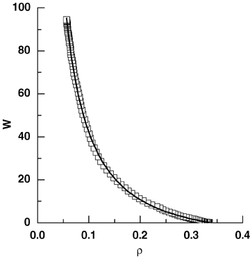
The dynamic self-thinning line in population with 29 785 initial plants.The curve is fitted using Equation 23.
| Type of the self-thinning | −β | k |
|---|---|---|
| Upper boundary linea | −1.349 ± 0.020 | 4.537 ± 0.140 |
| Dynamic thinning line in the population with 29 785 initial plantsb | −0.935 ± 0.605 | 13.238 ± 63.754 |
| Virtual dynamic thinning linea | −1.290 ± 0.007 | 3.120 ± 0.053 |
- a−β and k are from Equation 1; b−β and k are from Equation 23.
Virtual dynamic thinning line and the upper boundary line
Because plants in populations with the same initial size and hexagonal spatial pattern reached the largest sizes at the end of the simulation period, such populations were used to obtain the upper self-thinning boundary line. Density-dependent mortality occurred in four populations with the highest initial densities among the seven such populations. Combinations of density ρ and the corresponding largest mean plant biomass w are fitted well using Equation 1. The values of exponent −β and coefficient k are shown in Table 2 in detail.
The seven random populations were used to study the virtual dynamic thinning line defined by Equations 2 and 3. The w-ρ combinations on the virtual dynamic thinning line are well described with Equation 1 (Figure 8), and the exponent −β and coefficient k in the regression are shown in Table 2. The upper boundary line and the virtual dynamic thinning line are also plotted in Figure 6 on log-log scales. The upper boundary line lies above and is slightly steeper than the virtual dynamic thinning line, and dynamic thinning lines approach asymptotically the virtual dynamic thinning line as initial density gets higher and as competition goes on (Table 2, Figure 6). We also found in our study that the slopes and intercepts of the upper boundary line and the virtual dynamic thinning line were closer as initial spatial and size patterns were more uniform.
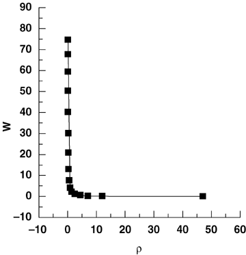
The virtual dynamic thinning line.The curve is fitted using Equation 1.
Discussion
Model selection
There are two main groups of individual-based models used in studies of the dynamics of plant populations: fixed-radius neighborhood models and zone-of-influence-like models, and the latter also include ordinary zone of influence (ZOI) models, ecological field models and field-of-neighborhood (FON) models. Fixed-radius neighborhood models (Pacala and Silander 1985; Pacala 1986, 1987; Zhang et al. 1989; Mabvurira and Miina 2002) are pioneer individual-based models. In these models, each plant is the center of a fixed-radius circle, and other plants within this circle are neighbors that compete with and influence the performance of the central plant. Fixed-radius neighborhood models are so simplified that they are seldom used now. Ordinary ZOI models (Wyszomirski 1983; Miller and Weiner 1989; Wyszomirski et al. 1999; Weiner et al. 2001) also assume a circular area around each plant, but the area increases as the plant grows and the meaning of the area is explicit: a plant obtains resources over the zone. If the ZOIs of two plants overlapped, they compete for the resources within the overlapping area. One shortcoming of ZOI models is that the influence intensity of a plant in the ZOI does not change. If the overlapping area of two plants remains unchanged, the distance between them does not matter, imagining ZOI of a smaller plant completely within that of a larger plant. Ecological field models (Wu et al. 1985; Mou et al. 1993; Li et al. 2000) and FON models (Berger and Hildenbrandt 2000) can be regarded as the recent developments of ZOI models. These models are similar, but the concept of FON provides more mechanistic resolution and less complexity than the ecological field theory. In these models, not only geometry of interaction but also intensity of interaction over space is defined. FON models have been used to study self-thinning (Berger et al. 2002; Berger and Hildenbrandt 2003), productivity (Berger et al. 2004), and size structures in monocultures (Bauer et al. 2004).
The objective of this study was to evaluate the relationship between the upper boundary line and the virtual dynamic thinning line. The main resource competed for among plants is assumed to be sunlight, and competition for light is asymmetric (Cannell et al. 1984; Weiner and Thomas 1986; Kikuzawa 1999). Taller plants preempt the sunlight and suppress the performances of underlying individuals, but shorter plants cannot shade taller plants. If a neighbor of a plant is defined as the suppressor of the plant, then a very tall plant is a neighbor of a very little plant nearby, but the little plant has little influence on the tall plant and cannot be called a neighbor of the tall plant. We wanted a model with such neighborhood definition as an intrinsic feature when we started this study. In ordinary ZOI models and FON models, plants are always mutual neighbors, so they were not used directly. Adler (1996) also developed an individual-based model to study the self-thinning rule, and we also evaluated his model. Adler's model is elegant when used to study the upper boundary line, but the “effective number” used in the model is less than or equal to the census number, with equality only when all plants have the same size. Adler's model cannot be used to get the virtual dynamic thinning line which is derived from the C-D effect, so it could not be used in this study. For our purposes, we developed a spatially explicit, individual-based model based on the “area of suppression” (AOS) concept. In the AOS model, intensity of competition between two plants depends on their relative sizes and the distance as in the FON approach, but plants influence each other directly, not through the resources in the overlapping area of ZOIs, as in traditional neighborhood models. We use the suppression index other than the resource substitution of ZOI for ease of definition of one-sided AOS and for a less intensive computing workload. Because the AOS of a plant is used just to identify the plants whose performances are suppressed by the plant, it holds the simplicity and computing efficiency of traditional neighborhood models. The allometric relationships of h-D and m-D are incorporated into the AOS model to make a more realistic model plant species. In our study, the C-D effect in simulated plant populations conformed well to Hagihara's model and findings in self-thinning Pinus densiflora and P. massoniana stands (Xue and Hagihara 1998, 2002), and dynamic thinning lines conformed to previous studies (e.g. Zeide 1987; Adler 1996) and were well described with Ogawa's model. It seems that the AOS model can conform well to empirical and theoretical equations (Hagihara's equation of the C-D effect and Ogawa's model of dynamic thinning line) given appropriate values of the parameters.
Possibility of using the virtual dynamic thinning line as the upper boundary line
Xue and Hagihara (1998) found that, in self-thinning P. densiflora stands, data points under the asymptotic density condition moved along a line with a slope slightly less steep than −3/2 and then along a line with a slope of ca. −3/2. It seems there may be a relationship between the virtual dynamic thinning line and the self-thinning upper boundary line. But they did not provide the exact slope of the virtual dynamic thinning line, and they did not discuss further the relationship between the two lines. When Xue and Hagihara (2002) studied the C-D effect in self-thinning P. massoniana stands, they also found that data points on the virtual dynamic thinning line first moved along a slope of ca. −1.2, and then reached the position of the self-thinning line with a slope of ca. −1.8. They explained that the difference in the results was because of different ages, indicating the complexity in field studies. We tried to find the possible relationship between the virtual dynamic thinning line and the upper boundary line from the perspective of a general model species for simplicity. In our study, the virtual dynamic thinning line and the upper boundary line are both straight lines on log-log scales and the slopes are almost the same values with only very little difference (0.059). We found in this study that the difference would be even less if there were more data points using to fit the upper boundary line and initial spatial and size patterns in the populations used to derive the virtual dynamic thinning line were more uniform. Although Table 2 shows that the exponent of the upper boundary line, −1.349, was not significantly different from −4/3 and different significantly from −3/2, this does not mean −4/3 is better than −3/2. We did not study the accurate self-thinning exponent in this study, and the exponent −1.349 may be the result of the parameter settings. Figure 6 shows that the intercept of the virtual dynamic thinning line is less than that of the upper boundary line. This difference in intercept may be because of different initial plant size and spatial patterns. The upper boundary line was obtained as plants grew with unique initial size and uniform (hexagonal) initial spatial distribution pattern. Under this condition, plant individuals were influenced at the same level, and the maximum mean plant biomass at a given density was the largest. While plants in the seven populations used to derive the virtual dynamic thinning line grew with normalized initial sizes and random spatial patterns. Under such conditions, the mean plant biomass in a population cannot reach the ideal largest value, so does the mean plant biomass in the virtual population used to fit the virtual dynamic thinning line. If populations are established with the plants, which are of more similar size and distributed more uniformly at the beginning of population development, the virtual dynamic thinning line will lift up closer to the upper boundary line.
The results of our study also show the difference among the upper boundary line, the dynamic thinning line and the virtual dynamic thinning line. The upper boundary line can only be derived from ideal populations with uniform initial size and spatial distribution, so the upper boundary line may be regarded as a theoretical upper boundary of combinations of mean plant biomass and density in self-thinning populations. But in experimental and field studies, it is hard to get appropriate data to fit the right upper boundary line, and this may partly be the reason why there are different values of the self-thinning exponent in the published reports. The dynamic thinning line is a population-specific line, which describes the time-trajectory of combinations of mean plant biomass and density in a given population as density-dependent mortality occurs. Dynamic thinning lines gradually approach but cannot reach the upper boundary line with the self-thinning process. Because plants are unmovable and there may be gaps in populations, the mean plant biomass in a population at a density does not always reflect the capacity of environments, and different populations have different dynamic thinning lines. The virtual dynamic thinning line is derived from the C-D effect as initial plant density tends to be positive infinity, so it is also a theoretical line like the upper boundary line. If there were no canopy gaps and density-dependent mortality occurred at any time in the population with infinite initial density, the mean plant biomass at any density would be regarded as an environmental characteristic, and then the virtual dynamic thinning line would be the same as the upper boundary line. In our study, it seemed that the virtual dynamic thinning line tended to be used as the upper boundary line in simulated plant populations given appropriate parameter values and as initial spatial and size patterns tended to be uniform.
Because the virtual dynamic thinning line bridges the gaps between the C-D effect and self-thinning, and between the dynamic thinning line and upper boundary line, it combines static and dynamic aspects of intraspecific competition into one whole body and it should be treated more seriously than ever. However, although Xue and Hagihara mentioned the relationship between the virtual dynamic thinning line and the upper boundary line when they studied the C-D effect in two self-thinning pine species, researchers have seldom studied the relationship. There are two dominating values, −3/2 and −4/3, of the self-thinning exponent in plant populations, and identifying which is more accurate and eventually identifying the underling mechanism is still one of the concerns of plant ecologists. But because of the ideal conditions exposed in this study, it is hard to derive the accurate upper boundary line by fitting directly to experimental or field data. If the relationship between the virtual dynamic thinning line and the upper boundary line is corroborated, then we can obtain the upper boundary line through the virtual dynamic thinning line without worrying about whether a data point is from a population with full density, avoiding the subjectivity in data selection as in traditional self-thinning studies. In our study, it seemed that the virtual dynamic thinning line could act as the upper boundary line in simulated plant stands given appropriate parameter values. The results of our study should be examined with further well-controlled experiments investigating the virtual dynamic thinning line. These experiments should pay attention to initial spatial and size patterns, which influence slightly the similarity of the virtual dynamic thinning line and the upper boundary line as revealed in our study.
Materials and Methods
In our model, we assign conventional units to measures of mass, area and time for ease of interpretation; however, these units are essentially arbitrary and should not be taken literally. The virtual experimental field was a 300 m × 300 m plain and homogeneous square. In order to avoid edge effects, only the plants in the central 100 m × 100 m region were “measured”. The embedded approach was used in this model, because it was found to be more realistic than the torus, linear expansion or reflection methods (Haefner et al. 1991). Simulated plant populations developed for 100 years at seven initial densities, with 7 360, 9 078, 12 932, 16 560, 20 064, 25 950 and 29 785 plants in the whole field, and in two initial spatial patterns, random or uniform (hexagonal). Plant growth equations were discretized using the fourth-order Runge-Kutta algorithm with a step interval of 0.2 year, and data were collected once a year (every five steps). Initial biomasses (m0) were 0.1 kg while deriving the upper boundary line, and distributed normally with a mean of 0.1 kg and a standard deviation of 0.015 while studying the dynamic thinning line and the virtual dynamic thinning line. For the parameters in the AOS model, we investigated the parameter space, but we just provided one set of parameter values in the present study for simplicity and brevity. Asymptotic biomass M was set to 100.0 kg for simplicity, and the value of r assured that biomass m reached approximately M at the end of the simulation period. Exponent q in the m-D allometric relationship was set to 2.67 according to Enquist et al. (1998), close to findings of previous studies (Osawa and Allen 1993; Sackville Hamilton et al. 1995; Yang and Titus 2002). Exponent b in the h-D allometric relationship was set to a value based on the findings of Weiner and Fishman (1994). Coefficients a in h-D and p in m-D relationships were set to values so that the maximum height and stem diameter of a plant reach about 8 m and 30 cm, respectively, when the plant grows in isolation. These scales seem to be appropriate in consideration of the size of the experimental field. Other parameters, i.e. c, k, e, j, were set to values so that plants have AOSs of proper size and die at certain density threshold. This specific point in parameter space gives us a general model species, considering biological reality and computing workload at the same time. Another reason we do not discuss the parameter space in this paper is that there exist parameter values just because of mathematical reasonability. For example, a condition that the asymptotic height is 100 m is reasonable in the model itself, but does not seem appropriate in a 300 m × 300 m experimental field. Table 1 lists parameter values for Equations 5, 6, 12, 13, and 16 in detail.
| Parameter | Description | Value |
|---|---|---|
| a | Allometric coefficient in Equation 5 | 30.08 |
| b | Allometric exponent in Equation 5 | 1.10 |
| p | Allometric coefficient in Equation 6 | 2 489.35 |
| q | Allometric exponent in Equation 6 | 2.67 |
| c | Coefficient in Equation 12 | 20.00 |
| r | Maximum relative growth rate in Equation 13 | 0.13 |
| M | Asymptotic plant mass in Equation 13 | 100.00 |
| k | Coefficient in Equation 13 | 30.075 |
| e | Coefficient in Equation 16 | 2.00 |
| j | Coefficient in Equation 16 | 0.01 |
Hagihara's model (1999) of the C-D effect in self-thinning populations and Ogawa's equation (2005) of a dynamic thinning line were used to validate the AOS model. These equations were chosen because: (i) Hagihara's model is suitable in self-thinning populations; (ii) Ogawa's equation incorporates some earlier models (Shibuya 1995; Hagihara 1998); and (iii) these equations describe the dynamics of self-thinning populations in static and dynamic aspects, respectively, and combination of these equations can effectively validate a plant competition model.
The output of our model consisted of the biomasses, heights and locations of all the plants in the central 100 m × 100 m region over time. The density and mean plant biomass of the plants alive in each population were calculated, and then the upper boundary line, dynamic thinning lines, the C-D effect and the virtual dynamic thinning line were analyzed. Because our simulations run in the deterministic mode, least square regression (LSR) methods other than principal components analysis (PCA) or reduced major axis (RMA) regression were used to analyze data. Nonlinear regression method based on the Levenberg-Marquardt algorithm of Origin 6.1 was used to fit simulation data.
To test the effects of random initial spatial pattern and normalized sized distribution, selected runs were repeated five times with different random number seeds. Variation between these replicates was so small that replication of other runs was cancelled.
The complete source code in C of our model will be provided on request, and researchers are invited to use it for further studies.
(Handling editor: Jian-Xin Sun)


