Flow dynamics and characterization of a cough
Abstract
Abstract Airborne disease transmission has always been a topic of wide interests in various fields for decades. Cough is found to be one of the prime sources of airborne diseases as it has high velocity and large quantity of droplets. To understand and characterize the flow dynamics of a cough can help to control the airborne disease transmission. This study has measured flow dynamics of coughs with human subjects. The flow rate variation of a cough with time can be represented as a combination of gamma-probability-distribution functions. The variables needed to define the gamma-probability-distribution functions can be represented by some medical parameters. A robust multiple linear regression analysis indicated that these medical parameters can be obtained from the physiological details of a person. However, the jet direction and mouth opening area during a cough seemed not related to the physiological parameters of the human subjects. Combining the flow characteristics reported in this study with appropriate virus and droplet distribution information, the infectious source strength by coughing can be evaluated.
Practical Implications
There is a clear need for the scientific community to accurately predict and control the transmission of airborne diseases. Transportation of airborne viruses is often predicted using Computational Fluid Dynamics (CFD) simulations. CFD simulations are inexpensive but need accurate source boundary conditions for the precise prediction of disease transmission. Cough is found to be the prime source for generating infectious viruses. The present study was designed to develop an accurate source model to define thermo-fluid boundary conditions for a cough. The model can aid in accurately predicting the disease transmission in various indoor environments, such as aircraft cabins, office spaces and hospitals.
Introduction
Transmission of infectious respiratory diseases has always been a topic of wide interests and has received attention from various disciplines for decades (Morawska, 2006). The transmission can happen through direct and indirect contacts or could be airborne. The transmission may take place through the droplets carrying the infectious viruses. Common airborne diseases are cold and influenza and severe ones are Acute Respiratory Syndrome (SARS) and avian flu. The Spanish flu of 1918–1919 (H1N1) was by far the most lethal flu pandemic of the 20th century. According to the World Health Organization (WHO) estimates, it infected about one-quarter of the global population and took the lives of more than 40 million people (WHO, 2002). A pandemic of avian flu among humans could cost the global economy $800 billion a year (World Bank, 2005). Not only avian flu could be deadly; there were 8098 people infected by SARS and 774 of them died according to statistics from the WHO (2002). The epidemic caused significant social and economic disruption in areas with sustained local transmission of SARS. As people spend most of their time at indoor workplaces, they would very likely be infected by flu or other airborne infectious viruses if there is a pandemic. This indicates a clear need for the scientific community from various disciplines to accurately predict and control the transmission of airborne diseases.
Airborne transmission starts from infectious viruses exhaled from an infected person (Cole and Cook, 1998). Then the viruses are transported in the air and finally inhaled by a susceptible person. Some have investigated the virus transportation (Holmes and Morawska, 2006) in air, but there is no comprehensive literature on exhalation and inhalation characterization. Transportation of airborne viruses is predicted using Computational Fluid Dynamics (CFD) simulations (Holmes and Morawska, 2006) or using benign bacterial virus and biological air sampling technique (Sze To et al., 2008). But CFD simulations are often used as they are inexpensive in comparison with the experiments. They need flow-thermal boundary conditions from the source of infectious viruses. The boundary conditions for exhalation are as follows:
- •
Flow rate and direction
- •
Mouth or nose opening area
- •
Temperature
- •
Size distribution of the virus droplets and quantity of virus in the droplets.
These parameters are transient and can have considerable variation among people. The CFD simulations (Zhao et al., 2005; Zhu et al., 2006a,b) for dispersion predictions have treated these boundary conditions as constant flow rate with assumed direction, temperature, a ballpark number for the area of the mouth or nose opening. Accurate boundary conditions are important for precise prediction of disease virus transmission.
Exhalation modes include coughing, sneezing, talking, or breathing. Coughing and sneezing processes are the major sources of contaminants as they have higher droplet concentration (Duguid, 1945) compared with the others. But as coughing is a common symptom for most respiratory infections, the present study is focused on developing a model to prescribe the boundary conditions for the coughing process. There is substantial literature on cough droplet size distribution (Chao et al., 2009; Duguid, 1945; Fairchild and Stamper, 1987; Fennelly et al., 2004; Hersen et al., 2008; Morawska et al., 2009; Papineni and Rosenthal, 1997; Yang et al., 2007) and exhaled air temperature (Hoppe, 1981). Hence this study limited the scope to the flow dynamics of a cough, i.e. flow rate, flow direction, and the area of mouth opening during a coughing process.
State of the art
Exhale airflow rate and direction from a cough
Figure 1 shows the typical flow generated from a cough over time. Information about cough flow rate is available from the literature (Leiner et al., 1966; Mahajan et al., 1994; Singh et al., 1995), such as Cough Peak Flow Rate (CPFR), Cough Expired Volume (CEV) that is the area under the curve, and Peak Velocity Time (PVT). The information is of great medical interests (Lamb et al., 1993), but it is not useful as boundary conditions in CFD simulations.
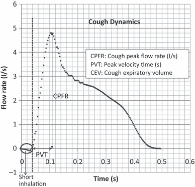
Cough flow rate variation with time
However, the information provides good insight of the flow behavior of a coughing process. Leiner et al. (1966) correlated CPFR with the height and age of human subjects through a regression analysis. Mahajan et al. (1994) further developed relations between CPFR, CEV and PVT. Later, Singh et al. (1995) corrected the relationship between CPFR and PVT for different genders and found the difference caused by the larynx size in male and female. The total cough volume measured by Zhu et al. (2006b) had a variation of 0.8–2.2 l with an average of 1.4 l which actually was the low end as compared with that from Mahajan et al. (1994), who observed a variation of up to 5 l with an average of about 3 l. Although these studies gave some information on cough, they did not quantify the dynamics of the cough profile.
On the contrary, there were a number of studies visualizing the coughing process that could be used to create boundary conditions for CFD simulations. Jennison (1942) visualized cough through high speed photography using strobe (Edgerton and Barstow (1959)). Their main emphasis was on droplet size distribution, but he also revealed qualitatively the droplet dispersion to 2–3 feet from mouth. Settles et al. (1995) captured the thermal plume coming out of a cough through Schlieren imaging. But none of these studies could characterize the transient process or direction of the jet. Particle Image Velocimetry (PIV) (Afshari et al., 2002; Badeau et al., 2002; Chao et al., 2009; VanSciver, 2005;Zhu et al., 2006a,b) measurements were also performed to capture the flow field. Mahajan et al. (1994) pointed out that the PVT was in the order of a few milliseconds. Hence to capture the cough jet variation and its direction, it becomes essential to have a high frequency of measurements. PIV measurements by Afshari et al. (2002) and Badeau et al. (2002) were done at an interval of 67 ms. The interval was too large and so the details of flow may not be captured. Chao et al. (2009) investigated the maximum and average velocities, but the velocity variation with time was not studied. The PIV studies by VanSciver (2005) gave detailed flow information but with an even large interval of 267 ms. The efforts by Zhu et al. (2006b) were also with a large interval of 70 ms. Therefore, none of these studies could be used to characterize the direction of a cough jet for CFD simulations. The measurements of the flow rate and direction must be performed with a frequency of 100 Hz or higher.
Mouth opening area during a cough
The area of mouth opening is required to obtain the velocity from the flow rate. The PIV studies by Zhu et al. (2006b) indicated the peak cough velocity varied from 6 to 22 m/s with an average of 11.2 m/s. To our best knowledge little experimental studies were on the area of mouth opening during a cough. Most researcher assumed (Zhao et al., 2005; Zhu et al., 2006a,b) the area to be a few square centimeters.
Measurement methods
The present study measured flow rates, flow directions and mouth opening areas of coughs. A spirometer based on Fleish type pneumotachograph (Bongers and O’Driscoll, 2006; Sancho et al., 2004) was used to measure the cough flow rates generated over time with a frequency of 330 Hz. The spirometer consists of numerous capillary tubes in parallel and gives the flow proportional to the pressure drop. It is based on Poiseuille’s Law, which states that, under capillary conditions in a straight rigid tube, flow is proportional to pressure loss per unit length. The flow directions were visualized through moderate-speed photography (120 Hz) with 1 Mega Pixel resolution. Cigarette smoke was used as seeding fluid. The cigarette smoke particle size is about 0.2 μm (Klepeis and Nazaroff, 2002) in diameter and the measured temperature of the cigarette smoke was close to exhaled air temperature. Thus, the exhaled smoke jet should closely follow the cough air jet profile. The mouth opening areas were measured through the moderate-speed photography (120 Hz). All the measurements were conducted with vertical head posture as shown in Figure 1. The head posture may affect the flow rate and flow direction in particular. But as the velocities during a cough are high, gravity effects may be negligible and the direction with respect to mouth may not change significantly.
All the measurements were performed over 12 female and 13 male subjects to obtain realistic flow features with an approval from the Institutional Review Board for human subject experimentation. Normal healthy subjects were recruited for the study. The subjects were first given an overview of the research and were told about the risk involved in the measurements. Every subject signed a consent form before proceeding for the measurements.
The flow rate measurements were done by placing a mask on subject’s face. The mask had ports for mouth and nose and the ports were connected to a filter then further to the spirometer as shown in Figure 2.
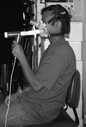
A subject with a mask holding the spirometer during test
Two types of flow measurements, single cough and sequential cough, were conducted. The single cough coughed just once, while sequential cough coughed twice. Each test was repeated three times for every subject.
The flow visualization study was performed on smoker subjects. A light source was placed beneath a subject face to throw light upwards. The light source along with a dark background helped the flow visualization. The subjects were asked to exhale smoke out through coughing.
The measurements of mouth opening area were performed over eight male and eight female subjects. The subjects were asked to cough and the front views close to their lips were captured for the whole event.
Results
This section presents the experimental results obtained from this investigation.
Flow rate of a cough
The flow rate characteristics of a cough are to develop a simple mathematical model describing the boundary conditions for CFD simulations.
Single cough. Figure 1 shows the flow rate generated from a typical cough over time from a subject. The results indicate that the cough began with a very short inhalation (<1% of the total exhaled air volume), a very high acceleration afterwards in exhalation and subsequently a decay. The inhalation volume was very small and may be neglected.
Figure 3 illustrates the transient flow of a cough for all the subjects studied. A large variation existed among the subjects. For example, the difference between the maximum and minimum values of CPFR, CEV and PVT for the male subjects was about 200, 300 and 100%, respectively. It is to be noted that the figure does not show inhalation of a coughing process. The total inhaled volume during a cough was less than a percent of the total exhaled volume during a cough. The velocity during the inhalation period was also low. Table 1 summarizes the variation range of the CPFR, PVT and CEV for the subjects who are very diversified Thus, the cough flow characteristics from a subject can not be used to represent the whole population that means a standard cough does not exist.
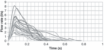
Cough flow rates for the 25 subjects
| Male | Female | |
|---|---|---|
| CPFR | 3–8.5 l/s | 1.6–6 l/s |
| CEV | 400–1600 ml | 250–1250 ml |
| PVT | 57–96 ms | 57–110 ms |
 (1)
(1) (2)
(2) (3)
(3) (4)
(4)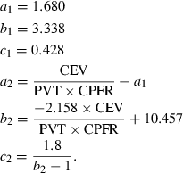 (5)
(5)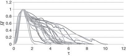
Dimensionless cough flow rates from the 25 subjects
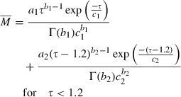
Figure 5 compares the measured flow rate with the fitted one obtained from Equations 3 and 4 for a subject. Such a good agreement was found for all the subjects.
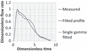
Comparison of the flow rate calculated by Equations 3 and 4 for a single cough from a subject with the measured data
It is to be noted that the CPFR, PVT, and CEV are unknown for a new subject. In order to apply the two equations to a new subject, it is essential to link these variables to the subject’s characters, such as height, weight, and gender. Our regression analysis by the solid lines shown in Figure 6 indicates that these medical parameters were inter-related. Figure 6a,b show the variation of the CEV with the CPFR for the male and female subjects, respectively. The figures show a positive correlation between all the parameter (r > 0.5, P < 0.005 for all). Since the CEV increases with the CPFR, this implies that the higher the peak flow rate the higher would be the total volume exhaled. The CPFR for the female subjects were lower than that for the male subjects. Mahajan et al. (1994) proposed using a single equation to correlate the CEV with the CPFR for both genders. As shown in Figure 6, their regression lines deviate significantly from our data. Our two regression lines that distinguish the genders fit the best to the data.

The relationship between CEV and CPFR for (a) male subjects and (b) female subjects
Similarly, Figure 7a,b show the variation of the PVT with the CPFR for the male and female subjects, respectively. The results again indicate that the PVT increased with the CPFR. The PVT for the female subjects was higher than that for the male subjects. This could be attributed to the difference in their larynx sizes as indicated by Singh et al. (1995). The slope of the PVT vs. the CPFR variation is similar to that obtained by him, but the intercept is higher by about 50 ms in our measurements. Our measurements were performed at 330 Hz and can capture the initial period, which could have got missed out in previous studies.
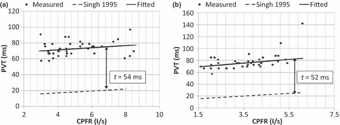
The relationship between PVT and CPFR for (a) male subjects and (b) female subjects
 (10)
(10) (11)
(11)The two equations can calculate the CPFR with an error no greater than 20% by comparing it with the data in our database. The equations indicate that the CPFR increases with the height and weight of the subject.
From the physiological information such as the height, weight, and gender, the CPFR can be calculated using Equations 10 and 11. The CEV and PVT can be calculated from the CPFR using Equations 6–9. With the CPFR, CEV, and PVT, the dimensionless flow rate can be obtained from Equations 3 and 4. Equations 1 and 2 can be utilized to convert the dimensionless flow rate into the dimensional one. Hence, the flow rate over time for a single cough can be obtained from the physiological information.
Sequential cough. A sequential cough is defined one cough followed immediately by the other. Figure 8 shows the flow generated for a sequential cough from a subject. The flow behavior for the two coughs in the sequential cough was similar to that of a single cough and can also be described by Equations 3 and 4. The first cough closely followed the features of a single cough, while the second one was a scaled down of the first one. Tables 2 and 3 compare the sequential coughs with the single coughs from the male and female subjects, respectively. The PVT for the two coughs in the sequential coughs was approximately the same as that of the single coughs, while the CPFR and CEV for the second cough were approximately 0.5.–0.6 times of the single coughs.
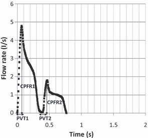
Flow rate over time for a sequential cough from a subject
| Correlation with single cough | |||||||||
|---|---|---|---|---|---|---|---|---|---|
| CPFR | PVT | CEV | |||||||
| r | P | Correlation | r | P | Correlation | r | P | Correlation | |
| First cough | 0.77 | <0.001 | 1.008 × CPFR | 0.58 | <0.001 | 1.105 × PVT | 0.6 | <0.001 | 0.8184 × CEV |
| Second cough | 0.53 | <0.001 | 0.602 × CPFR | 0.33 | <0.001 | 0.9568 × PVT | 0.45 | <0.001 | 0.602 × CEV |
| Correlation with single cough | |||||||||
|---|---|---|---|---|---|---|---|---|---|
| CPFR | PVT | CEV | |||||||
| r | P | Correlation | r | P | Correlation | r | P | Correlation | |
| First cough | 0.8 | <0.001 | 1.038 × CPFR | 0.7 | <0.001 | 1.107 × PVT | 0.63 | <0.001 | 0.8613 × CEV |
| Second cough | 0.7 | <0.001 | 0.6335 × CPFR | 0.51 | <0.001 | 0.8697 × PVT | 0.55 | <0.001 | 0.5294 × CEV |
Thus, the CPFR, PVT, and CEV for the first cough can be obtained from Equations 6–11, while those for the second cough should be corrected with Tables 2 and 3. The flow rate can then be obtained by Equations 3 and 4 for the two coughs.
Flow direction of a cough
The flow direction of a cough was obtained from flow visualization. Figure 9 shows the sequence of images taken at 120 Hz for a typical cough process from t = 0 to 36/120 s. The first three images were for t = 0 to 3/120 s, when the mouth was closed. Then, the images were from t = 9/120 to 36/120 s at an interval of 1/120 s. At t = 9/120 s, the mouth completely opened up but the smoke came out after t = 11/120 s.
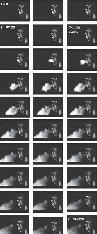
The side view of a cough process recorded with a frequency of 120 Hz
 (12)
(12) (13)
(13)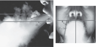
The cough jet direction from the side and front views
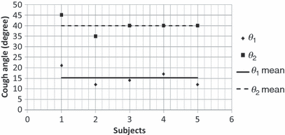
Variation in the two cough angles among all the subjects
The two mean angles can be used as boundary conditions for CFD modeling.
Mouth opening area
The mouth opening area is defined as the area between the lips during a cough. Figure 9 shows the sequence of images during a cough. Initially the mouth was closed and then opened up fully at t = 9/120 s. The mouth remained opened for the rest of the cough process. This can be further confirmed from the images of the front view for all the subjects. Figure 12 shows the mouth opening area over time for a subject. It can be seen that the mouth opening area was almost constant when there was flow from the mouth.
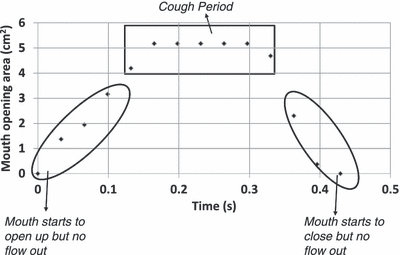
Change of mouth opening area during a cough
 (14)
(14) (15)
(15)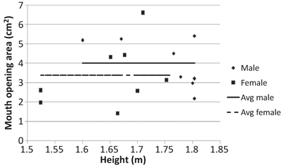
Variation in mouth opening area during a cough with the heights of all the subjects
Discussion
This investigation has developed a set of simple equations that can be used to generate boundary conditions (or a source model) for predicting infectious virus transport by CFD due to coughing. Our effort focused on the flow rate, flow direction, and air velocity that can be determined from flow rate and mouth opening area. The inputs required are height, weight, and gender of a person.
The boundary conditions required by CFD simulations should also include the temperature of the exhaled air and the droplet distribution. The study by Hoppe (1981) can be utilized to obtain the exhaled air temperature under various ambient temperature and humidity. He found that ambient temperature is the most influential parameter. There are a few studies on cough droplet size measurements (Chao et al., 2009; Duguid, 1945; Fairchild and Stamper, 1987; Fennelly et al., 2004; Hersen et al., 2008; Morawska et al., 2009; Papineni and Rosenthal, 1997; Yang et al., 2007). The measurements were done over healthy subjects (Chao et al., 2009; Duguid, 1945; Fairchild and Stamper, 1987; Hersen et al., 2008; Morawska et al., 2009; Papineni and Rosenthal, 1997; Yang et al., 2007) and the subjects infected by TB (Fennelly et al., 2004) and with cough and cold (Hersen et al., 2008). The latest measurements (Hersen et al., 2008; Yang et al., 2007) indicated that the droplet concentration was of the order of 106 and the size varied from 0.1 to 10 μm. The study by Yang et al. (2007) indicated a linear trend with mean cough flow rate. Hence by knowing the mean cough flow rate from our model, the droplet concentration can be obtained.
Conclusions
This paper reports our effort to characterize the flow behavior of cough. The flow rate, flow direction, and mouth opening area were measured for 25 human subjects, which could be used as boundary conditions in CFD simulations.
The flow rate can be defined as a combination of gamma-probability-distribution functions. The variables in the functions can be represented by medical parameter, i.e. CPFR, PVT, and CEV. These medical parameters are related to the height, weight, and gender of a person.
A sequential cough was found to be the combination of two single coughs. The first one behaved approximately the same as that of a single cough, while the second one was a scaled down version of the first one.
The cough flow direction was visualized through the moderate-speed photography using smoke. The flow direction did not vary very much among the subjects and can be determined by two angles.
The mouth opening area was constant during a cough. The mouth opening area varied among the subjects but without a clear correlation with the subject height. Hence this study proposed to use a mean mouth opening area during a cough.


