Pricing Survivor Derivatives With Cohort Mortality Dependence Under the Lee–Carter Framework
ABSTRACT
This article introduces cohort mortality dependence in mortality modeling. We extend the classical Lee–Carter model to incorporate cohort mortality dependence by considering mortality correlations for a cohort of people born in the same year. The pattern of cohort mortality dependence is demonstrated on the basis of U.S. mortality experience. We study the effect of cohort mortality dependence on the pricing of survivor derivatives. For this purpose, a survivor floor is introduced. To understand the difference between a survivor floor and other survivor securities, the valuation formulas for survivor swaps and survivor floors are all derived in detail and the effects of cohort mortality dependence on pricing survivor derivatives are investigated numerically.
INTRODUCTION
Longevity risk has become an increasingly important consideration for defined benefit pension plans and annuity providers, because life expectancy is increasing dramatically in developed countries. In 2007, exposure to improvements in life expectancy reached $400 billion for pension fund and insurance companies in the United Kingdom and United States (see Loeys, Panigirtzoglou, and Ribeiro, 2007). Therefore, finding a way to measure longevity risk and transferring the longevity risk away from the pension fund or annuity provider is of great interest to plan sponsors. Reinsurance, which represents a traditional means to transfer the longevity risk, can be expensive and involves a potential credit risk to the counterparty. In turn, many life insurance companies are less willing to buy reinsurance for their longevity risk. Instead, capital market solutions such as mortality-linked securities have emerged.
Blake and Burrows (2001) were the first to advocate the use of mortality-linked securities to transfer longevity risk to capital markets. They suggested that the governments should help insurance companies hedge their mortality risks by issuing survivor bonds whose coupon payments depend on the proportion of the population surviving to particular ages. The longevity bond launched by the European Investment Bank (EIB) was the first securitization instrument designed to transfer longevity risk but ultimately was not issued and remained theoretical. Furthermore, various new securitization instruments and derivatives for longevity risk, such as survivor swaps, survivor futures, and survivor options, have received great attention among academics and practitioners (Blake, Cairns, and Dowd, 2006; Blake et al., 2010; Dowd et al., 2006; Biffis and Blake, 2009). The first derivative transaction, a q-forward contract, was issued in January 2008 between Lucida1 and J.P. Morgan (Coughlan et al., 2007). In addition, the first survivor swap executed in the capital markets took place between Canada Life and a group of ILS and other investors in July 2008. In this context, the valuation of mortality-linked securities represents an important research topic for the development of capital market solutions for longevity risk.
The dynamics of underlying mortality indexes have important effects on valuing life insurance or mortality-linked securities. The Lee–Carter model (Lee and Carter, 1992) has proved an effective method for mortality forecasts, which Denuit, Devolder, and Goderniaux (2007) use to value longevity bonds. Cairns, Blake, and Dowd (2006) also propose a two-factor stochastic mortality model (hereafter denoted CBD model) for higher ages and examine the pricing of longevity bonds. The Lee–Carter and CBD models both project mortality rates based on age and period effects. Renshaw and Haberman (2006) extend the Lee–Carter model to consider cohort effects2 in mortality modeling. Cairns et al. (2009) quantitatively compare eight stochastic mortality models and demonstrate that the CBD model (Cairns, Blake, and Dowd, 2006) that incorporates a cohort effect fits data about English and Welsh men best, and Renshaw and Haberman's (2006) extension of the Lee–Carter model that also allows for a cohort effect provides the best fit for data pertaining to U.S. men. Thus, the cohort effect represents an important risk factor that governs the dynamics of mortality. The preceding models are all discrete mortality models. In addition to these discrete models, some mortality models have been built on a continuous basis, including those proposed by Milevsky and Promislow (2001), Dahl (2004), Biffis (2005), Dahl and Møller (2006), and Schrager (2006). Liao, Yang, and Huang (2007) assume that mortality follows a nonmean-reverting stochastic process for a single age, as proposed by Luciano and Vigna (2005), and examine tranching in mortality-linked securities with a product designed to transfer longevity risk. Wills and Sherris (2010) use the continuous time dynamics of the mortality rate to price and structure a longevity bond based on that used for a collateralized debt obligation. Thus, the existing literature focuses on longevity securitization and illustrates the structure and pricing for longevity bonds. In this research, we attempt to price survivor derivatives for which the claim is contingent, that is, the option-type contract. The insurer suffers exposure to the longevity risk only when annuitants live longer than predicted by the reference mortality rates. Thus, the insurer, as the protection buyer, can hedge longevity risk by purchasing a survivor floor where the contingent claim occurs only when the actual survival probability is higher than the projected survival probability. Similar to an interest rate floor, a survivor floor can be viewed as a series of European basket put options on mortality rates and protects the floor buyer from losses that would result from a decrease in mortality rates. Pricing a survivor floor is considered in this article.
Mortality independence traditionally has been assumed in mortality modeling, regardless of whether it uses continuous or discrete models. However, a person's mortality actually may be correlated with and result in mortality dependence, which exists in longevity risk at the aggregate level (Millossovich and Biffs, 2006). Loisel and Serant (2007) were the first to take into account interage and interperiod correlations in mortality modeling and propose a stochastic logit delta model as a multidimensional extension of the Lee–Carter model. They demonstrate that most stochastic mortality models that use either a collection of independent copies of the intensity process with zero correlation or a single stochastic process with perfectly positive correlation contradict empirical findings. The former model is simple, but it is not realistic, because a positive correlation exists and cannot be neglected. Shyu and Chang (2007) analyze the pricing of a tranched life insurance-linked security under mortality dependence. Their analysis suggests that Lin and Cox's (2005) independence assumption overestimates the premium of the equity tranche and underestimates the premiums of the mezzanine and senior tranches. Wills and Sherris (2010) also demonstrate the effect of age dependence on pricing longevity bonds. Therefore it is crucial, especially for pricing mortality-linked securities or survivor derivatives, to use flexible stochastic mortality models that capture the mortality dependence structure.
We extend the prior literature by introducing cohort mortality dependence to mortality modeling; the idea implies that the mortality rates of persons born in the same year (cohort group) are correlated. The Lee–Carter model has been widely applied to price mortality-linked security, but never with a consideration of the effect of cohort mortality dependence (Denuit, Devolder, and Goderniaux, 2007). Although Koissi, Shapiro, and Högnäs (2006) find the deviance residuals obtained by Lee–Carter model are identically distributed over ages and calendar years using the Nordic countries, Yang, Chang, and Yeh (2008) further find that the residuals projected by Lee–Carter model for the countries of France and Switzerland are not identically and independently distributed. To overcome the problem that the residuals may not be identically and independently distributed under the Lee–Carter model, this research provides the methodology to construct the cohort mortality correlation structure under the Lee–Carter model. The pattern of cohort mortality dependence is assessed using U.S. mortality experience based on Human Mortality Database (HMD, ). To study the impact of cohort mortality dependence on the pricing of survivor derivatives, we introduce a survivor floor, which involves the exchange of a fixed series of payments for a series of basket survivor options. For comparison, we also demonstrate the effect of cohort mortality dependence on pricing a survivor swap. We take the cohort mortality dependence into account to derive the analytic pricing formulas for both survivor swaps and survivor floors. We also examine the effect of cohort mortality dependence on the risk premium numerically. The incorporation of cohort mortality dependence emerges as very important for pricing survivor derivatives.
In the next section, we present a Lee–Carter model with age-specific error terms and introduce cohort mortality dependence. We derive cohort mortality correlations related to survival probability and investigate cohort mortality dependence with empirical data. In turn, we introduce stochastic mortality rates with multivariate Wang transformation, describing the design and pricing of survivor derivatives. In the numerical analysis section, we provide empirical and numerical analyses to emphasize the impact of cohort mortality dependence on the valuation of the survivor floor. Finally, we draw some conclusions from our findings.
LEE–CARTER MODEL WITH COHORT MORTALITY DEPENDENCE
The Model
 , where P is the physical probability measure, N is a positive integer, and
  is the information available at time t. Let mx, t denote the central death rate at age x during calendar year t. To introduce the cohort mortality dependence in modeling longevity risk, we use the classical Lee–Carter model, which is
 (1)
(1) and
and  , respectively, to ensure the model identification. This structure is designed to capture age and period effects, such that the ax coefficients incorporate both the main age effects averaged over time and the actual force of mortality change according to an overall mortality index kt, modulated by an age response bx. The error term ex, t reflects particular age-specific historical influences that are not captured by the model. In the classical Lee–Carter model, the error term is assumed to be a particular discrete-time Markov stochastic process, with mean change of 0 and a variance rate of
  . In other words, the change of
  , which is independent of
  , has a normal distribution with mean zero and variance
  . Different from the original Lee–Carter model, we additionally assume that the correlation coefficient between
  and
and  is equal to
  , which captures age-specific mortality dependence between an x-aged person and y-aged person and thus contributes to cohort mortality dependence.
 (2)
(2) ,
,  , and
, and  are the drift, AR, and MA parameters, respectively, with
  ; and
; and  , independent of et, is normally distributed with mean 0 and deterministic variance
  . In most applications, kt is well modeled as a random walk with drift or referred to as the ARIMA(0,1,0) model:
  . In this case, the forecasted kt changes linearly, and the corresponding forecasted mortality rate changes at a constant exponential rate. However, Lee (2000, p. 83) also suggests, “Sometimes a model of this general form, but with an added moving average term or autoregressive term, is superior.” We use the generalized ARIMA(p,1,q) model to describe the mortality forecast.
 ), can represent the sum of past mortality indexes prior to time t0, such that
 (3)
(3) (4)
(4) (5)
(5) ,
,  , and
, and  for
for  and
and  . The proof of Equation (3) appears in Appendix A.
 (6)
(6) (7)
(7) denotes the expected cumulative rate of x-aged mortality improvement under the physical probability measure P and satisfies
 (8)
(8) (9)
(9) , or the variance of the logarithm of
  conditional on time t0 information
  , satisfies
 (10)
(10) is the mortality index volatility of
  ;
;  is the age volatility of
  , n = 1, …, N; and
  takes the form:
 (11)
(11)Proof: Please see Appendix B.
 denote the 1-year survival probability that an x0-aged person in calendar year t0 reaches age x0 + 1. We assume that the age-specific mortality rates are constant within bands of age and time but may vary from one band to the next. Specifically, given any integer age x0 and calendar year t0, we suppose that
 (12)
(12) under a constant force of mortality assumption. Let
  denote the n-year survival probability that an x0-aged person in calendar year t0 reaches age x0 + n. We calculate the survival probability based on the cohort mortality rate,3 which is
 (13)
(13) , represents the arithmetic sum of the mortality rates.
 (14)
(14) , and
, and
 (15)
(15)If we divide An by Fn and refer to the result as  , Proposition 2 provides the first two moments of
  .
.
 denote the normalized An, to calculate the survival probability in Equation (13). Under the physical probability measure P, the first two moments of
  take the form:

 (16)
(16) denotes the cohort mortality correlation between ages x0 + i and x0 + j, based on the cohort to which a person aged x0 at time t0 belongs, which also corresponds to the cohort mortality dependence that we introduce.
The proof of Proposition 2 appears in Appendix C.
 . Under the Lee–Carter model, conditional on time t0 information
  , the cohort mortality dependence for people between the ages of x0 + i and x0 + j can be expressed as
 (17)
(17)Equation (17) shows that the cohort mortality correlation depends on the age-specific mortality correlation ( ) between an x0 + i-aged person and an x0 + j-aged person. In addition, according to Equations (10) and (11), different ARIMA models contribute to different AR and MA parameters, as well as
  and the variance
  , which then lead to different cohort mortality dependence structures. If we calculate the survival probability in Equation (13), according to Proposition 2, we find that mortality improvements among different ages exhibit cohort mortality dependence.
Empirical Investigation of Cohort Mortality Dependence
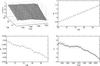
We employ U.S. mortality data from the HMD () to illustrate the pattern of cohort mortality dependence. For mortality data of 1933 through 2007, we use a close approximation to singular value decomposition method4 to find the parameter estimates of the Lee–Carter model. The pattern of empirical mortality rates and the fitted values of ax, bx, and kt appear in Figure 1. The mortality surface depicts the development of logarithm central death rates over calendar time; the downward slope of the time index kt reflects the trend of mortality improvement.
The structure of cohort mortality dependence under the Lee–Carter model depends on how we project the future mortality rates. Time series analysis is widely employed to model kt (Lee, 2000; Renshaw and Haberman, 2006; Denuit, Devolder, and Goderniaux, 2007). We also obtain the cohort mortality dependence by modeling the kt as an ARIMA(p,1,q) process (see Equation (2)). Thus, we examine various ARIMA(p,1,q) models and evaluate their fit, according to the Akaike information criterion (AIC)5 and the log-likelihood. Table 1 lists the parameters for different ARIMA(p,1,q) models and the corresponding AIC and log-likelihood. Clearly, for the United States mortality experience, the ARIMA(2,1,2) model6 is the most appropriate for describing the mortality index; ARIMA(0,1,0) offers worse performance, according to the AIC and log-likelihood values.7
| Parameter Estimation | Drift | AR(1) | AR(2) | MA(1) | MA(2) | AIC | Log-Likelihood |
|---|---|---|---|---|---|---|---|
| ARIMA(0,1,0) | −0.2411*** | 64.5969 | −63.5969 | ||||
| ARIMA(1,1,0) | −0.2930*** | −0.2182** | 63.7971 | −61.7971 | |||
| ARIMA(0,1,1) | −0.2419*** | −0.2257** | 63.6373 | −61.6373 | |||
| ARIMA(1,1,1) | −0.2550** | −0.0556 | −0.1789 | 64.6200 | −61.6200 | ||
| ARIMA(2,1,1) | −0.4098** | −0.5363 | −0.1891 | 0.2949 | 65.1621 | −61.1621 | |
| ARIMA(1,1,2) | −0.0382 | 0.8690*** | −1.2062*** | 0.4092*** | 63.3038 | −59.3038 | |
| ARIMA(2,1,2) | −0.4060*** | −0.7735*** | −0.2381** | 0.7503*** | 63.1936 | −59.1936 | |
| ARIMA(2,1,2) | −0.4571*** | −0.2186** | −0.6712*** | 0.5473* | 63.9651 | −59.9651 | |
| ARIMA(2,1,2) | −0.3832*** | 0.0759 | −0.8022*** | −0.2884** | 0.8148*** | 64.0709 | −59.0709 |
- ***, **, and * denote statistical significance at the 1%, 5%, and 10% levels, respectively.
| λ | Interest Rate = 0.01 | Interest Rate = 0.03 | Interest Rate = 0.05 | |||
|---|---|---|---|---|---|---|
| MC | RC | MC | RG | MC | RG | |
| 0.05 | 161.7867 | 161.7261 | 142.6636 | 142.6057 | 124.8491 | 124.7942 |
| (0.1027) | (0.0924) | (0.0827) | ||||
| 0.15 | 123.0427 | 122.9817 | 108.3699 | 108.3116 | 94.7051 | 94.6499 |
| (0.1033) | (0.0929) | (0.0832) | ||||
| 0.25 | 84.0766 | 84.0152 | 73.8629 | 73.8043 | 64.3598 | 64.30426 |
| (0.1039) | (0.0935) | (0.0837) | ||||
- Note: The MC column is the fair swap rate calculated by using Monte Carlo simulation with 1 million paths. The RG column is the fair swap rate calculated by applying Equation (37). Figures in brackets are the standard errors for Monte Carlo simulation.
| λ | Interest Rate = 0.01 | Interest Rate = 0.03 | Interest Rate = 0.05 | |||
|---|---|---|---|---|---|---|
| MC | RG | MC | RG | MC | RG | |
| 0.05 | 165.3933 | 165.4486 | 146.5108 | 146.5557 | 128.8840 | 128.9198 |
| (0.0936) | (0.0836) | (0.0743) | ||||
| 0.15 | 130.9774 | 131.0546 | 116.2175 | 116.2810 | 102.4199 | 102.4712 |
| (0.0884) | (0.0790) | (0.0701) | ||||
| 0.25 | 99.1985 | 99.2642 | 88.2550 | 88.3078 | 78.0013 | 78.0426 |
| (0.0808) | (0.0722) | (0.0642) | ||||
- Note: The MC column is the fair floor rate calculated by using Monte Carlo simulation with 1 million paths. The RG column is the fair floor rate calculated by applying Equation (38). Figures in brackets are the standard errors for Monte Carlo simulation.
| λ | Interest Rate = 0.01 | Interest Rate = 0.03 | Interest Rate = 0.05 | |||
|---|---|---|---|---|---|---|
| Cohort Mortality Independence | Cohort Mortality Dependence | Cohort Mortality Independence | Cohort Mortality Dependence | Cohort Mortality Independence | Cohort Mortality Dependence | |
| 0.05 | 159.8856 | 161.7261 | 141.0524 | 142.6057 | 123.4958 | 124.7942 |
| 0.15 | 121.0907 | 122.9817 | 106.7155 | 108.3116 | 93.3156 | 94.6499 |
| 0.25 | 82.0733 | 84.0152 | 72.1649 | 73.8043 | 62.9336 | 64.3043 |
- Note: The numerical results for cohort mortality independence are obtained by assuming that the cohort mortality correlations defined in Equation (17) are equal to 0.
| λ | Interest Rate = 0.01 | Interest Rate = 0.03 | Interest Rate = 0.05 | |||
|---|---|---|---|---|---|---|
| Cohort Mortality Independence | Cohort Mortality Dependence | Cohort Mortality Independence | Cohort Mortality Dependence | Cohort Mortality Independence | Cohort Mortality Dependence | |
| 0.05 | 160.3233 | 165.4486 | 141.6884 | 146.5557 | 124.3204 | 128.9198 |
| 0.15 | 122.1056 | 131.0546 | 107.9694 | 116.2810 | 94.7924 | 102.4712 |
| 0.25 | 84.6368 | 99.2642 | 74.9671 | 88.3078 | 65.9472 | 78.0426 |
- Note: The numerical results for cohort mortality independence are obtained by assuming that the cohort mortality correlations defined in Equation (17) are equal to 0.
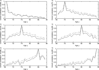
With the parameters in Table 1, we calculate the cohort mortality correlations between different ages based on Equation (17) using both the ARIMA(2,1,2) (solid line) and ARIMA(0,1,0) (dashed line) models. For illustrative purposes, Figure 2 only depicts the cohort mortality correlations for certain ages—66, 70, 75, 80, 85, and 89 with all other ages separately. It reveals two particularly important findings. First, the patterns of cohort mortality dependence for both ARIMA(0,1,0) and ARIMA(2,1,2) models are similar, but the cohort mortality correlations of the ARIMA(0,1,0) model are higher than those of the ARIMA(2,1,2) model, which means that the ARIMA model selection can affect cohort mortality dependence. Second, Figure 2 displays a remarkable phenomenon: the correlations between the mortality rates of younger ages and the mortality rates of older ages are lower, whereas those among older ages based on the same cohort are higher. For example, in the upper left-hand panel of Figure 2, the mortality correlations between persons aged 66 years and 80+ years are lower than 0.15. Therefore, a higher mortality rate at this age, such as might be due to accidents or catastrophic events (e.g., 2004 earthquake, tsunami), does not lead directly to higher mortality rates among older ages of the cohort. However, because most people die of natural causes, the mortality correlations at older ages should be higher than those in younger ages. In the lower right-hand panel of Figure 2, the cohort mortality correlation between ages 87 and 89 years equals 0.5296, and that between ages 88 and 89 years equals 0.4592.
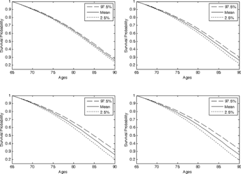
We further take cohort mortality dependence into account to reveal the pattern of future survival probabilities. For comparison purposes, we illustrate different cohort mortality correlation assumptions of 0, 0.3, 0.6, and 0.9 for different ages and plot the corresponding 95 percent confidence interval of the simulated survival probabilities for a person aged 65 in Figure 3. A cohort mortality correlation of 0 implies mortality independence. The higher the cohort mortality correlation, the more uncertainty is involved in the future dynamics of mortality. Thus, ignoring cohort mortality dependence might underestimate longevity risk. We study the impact of cohort mortality dependence on pricing survivor derivatives.
PRICING SURVIVOR DERIVATIVES WITH COHORT MORTALITY DEPENDENCE
Survivor Swaps Versus Survivor Floors
To investigate the effect of cohort mortality dependence on pricing survivor derivatives, we extend the literature by introducing a survivor floor for which the claim is contingent (i.e., an option-type contract). To clarify the mechanics of the survivor floor, we describe the survivor swap first and compare it with the proposed survivor floor. A survivor swap has been widely explored in the prior literature (Dawson, 2002; Blake, 2003; Dowd, 2003; Lin and Cox, 2007). Dowd et al. (2006) introduce the mechanism of a survivor swap for transferring longevity risk. A survivor swap is an agreement that involves the periodic exchange of a series of preset payments for a series of random mortality-dependent payments. On each payment date, the fixed-rate payer pays a preset amount, equal to the value of the notional principal multiplied by a fixed rate, and receives in return from the floating-rate payer a random mortality-dependent payment, equal to the value of the notional principal multiplied by the unexpected shock in survival probability (i.e., the difference between the actual survival probability and the reference survival probability). Thus, survivor swaps can be used to transfer the unexpected shock in mortality improvement. Down et al. point out that hedge is only as good as it is when the reference index is based is the insurer's own mortality experience. For more standardized reference indexes, if the expected reference indexes and insurers' own mortality experiences are highly correlated, the survivor swap can still hedge the insurer against a considerable amount of the aggregate mortality risk it faces.
 be the total number of annuities of an insurer issued to a cohort that consists of persons aged x0 at time t0. To transfer longevity risk, the insurer could purchase an N-year survivor swap at time t0 with a total nominal value
  , which is equal to the total number of annuity payments. The future actual payout to the annuitant at time t0 + n is estimated at time t0, denoted CFn and given by
 (18)
(18) represents the actual n-year survival probability for a person aged x0 at time t0 and we model
  using the proposed Lee–Carter model with cohort mortality dependence, as we described in the Lee–Carter model with cohort mortality dependence section.
 , which is given by
 (19)
(19) is the n-year survival probability for a person aged x0 at time t0 based on the reference mortality table used by the insurer. We assume the insurer used the mortality experience in year 2007 (HMD, ) for the reference mortality table.
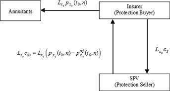
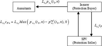
Let cS denote the fixed swap rate and cS n be the floating swap rate. The cash flows of a survivor swap for the fixed-rate payer and floating-rate payer are presented in Figure 4. At each payment date t0 + n,  , the insurer, which is also the longevity risk protection buyer, pays a prespecified fixed premium amount
  to a special purpose vehicle (SPV), which is the longevity risk protection seller, and sets up for this transaction and receives the floating payment amount,
 . In other words, the floating swap rate (cS n) equals to
  . After using the survivor swap, the insurer can effectively manage the time t0 + n aggregate cash outflow, equal to the scheduled payout
  plus the swap rate
  for
for  .
.
 , equal to the total number of annuity payments. Then cF denotes the floor rate and cF n is the reference rate. The fixed payment is calculated as
  , and the floating payment is calculated as
  . The contingent loss for the insurer occurs when the annuitants live longer than that predicted by the reference mortality rates. The contingent loss at time t0 + n can be expressed as
 (20)
(20)
 (21)
(21) (22)
(22) (23)
(23)In brief, both survivor swaps and the survivor floors can effectively hedge the longevity risk of the insurer. The main difference is that the floor is an option and requires more premiums to hedge longevity risk. Under the no arbitrage condition, the hedge cost for the survivor swap therefore should be lower than the hedge cost for the survivor floor; accordingly, the swap rate (cS) is lower than the floor rate (cF).
Multivariate Wang Risk Measure
 follows a Gaussian copula with a correlation matrix
  . A multivariate extension of the Wang transformation is
 (24)
(24) is the
  -variate standard normal distribution, and
  is the risk-adjustment parameter for the physical distribution of the jth variable,
  .
. . Because
  and
and  ,
,  , are normally distributed, the transformed distributions of
  and
and  ,
,  , based on the multivariate Wang transformation, equal
 (25)
(25) represents the risk-adjustment parameter for the physical distribution of an x0 + j-aged error term, and
  denotes the risk-adjustment parameter for the physical distribution of the mortality index. Therefore, the multivariate Wang transformation distorts the log-change in the x0 + i-aged mortality rate during calendar year t0 + n to another lognormal distribution.
 (26)
(26) denotes the expected n-period cumulative rate of x-aged mortality improvement under Q, as given by
 (27)
(27)Proof: Substituting Equation (25) into Equation (7), we can obtain Equations (26) and (27).
 ,
,
 (28)
(28) values and expected cumulative rate of x-aged mortality improvement for the physical probability measure P. Second, the x0 + i-aged force of mortality during calendar year t0 + n, conditional on
  , follows a new MA(n) process under the Wang risk measure Q, the MA order of which depends on the observed time span n. In addition, according to Proposition 3, we further express the risk-neutralized survival probability for the projected
  in the form of
 (29)
(29) ;
;  ;
;  is the modified Bessel function of the second kind with order
  ;
;  ;
;  ; and
; and  . We use the reciprocal gamma distribution proposed by Milevsky and Posner (1998a, 1998b) as an approximation of the state-price density of An to derive Equation (29), and the Proof of Equation (29) is shown in Appendix D. Q.E.D.
Pricing Survivor Swaps and Survivor Floors With the Wang Risk Measure Q
 ; r(t) is the risk-free rate. The price of a zero-coupon bond under the risk measure Q satisfies the following expression:
 (30)
(30) (31)
(31) , where
  is the sum of force of mortality rates ranging from age x0 to age x0 + n − 1 based on the reference mortality table. Note that
  . Thus, we can express the floating swap rate as
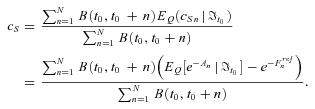
  . Under the assumption that the mortality rate and financial risk are independent, we can derive the fair swap rate as follows:
 (32)
(32) (33)
(33) and
and  into Equation (22), we obtain
 (34)
(34) .
. (35)
(35)Equation (32) implies that the fair swap rate is determined by the moment-generating function of An. Similarly, Equation (35) implies that the fair floor rate is determined by a series of basket put options on mortality rates with the payoff  , which is the survivor option. We use the reciprocal gamma distribution proposed by Milevsky and Posner (1998a, 1998b) as an approximation of the state-price density of An and thereby obtain an approximate closed-form expression for the fair valuation of survivor swaps and survivor floors.
 (36)
(36)Proof: Substituting Equation (29) into Equation (32), we can obtain Equation (36). Q.E.D.
 (37)
(37) (38)
(38)where  denotes the cumulative distribution of the gamma distribution evaluated at x.
Please see Appendix E for the proof.
NUMERICAL ANALYSIS
Fair Swap Rates and Floor Rates
We examine the effects of cohort mortality dependence on the valuation of survivor swaps and survivor floors. The assumption of cohort mortality dependence directly follows the projection using the ARIMA(2,1,2) model. We consider a person aged 65 years in 2007, that is, x0 = 65 and t0 = 2007. The maturity of the survivor floor is 25 years. Without loss of generality, we assume that the initial term structure is flat and the risk-adjustment parameters are equal, so  . We illustrate the result when
  is 0.05, 0.15, and 0.25 and when the initial term structure is flat at 1, 3, and 5 percent.
In Tables 2 and 3, we first examine the accuracy of the pricing formulas for both survivor swaps and survivor floors using simulations separately. For an interest rate of 3 percent and a risk premium of 0.15, the fair swap rate for a survivor swap is 108.3116 basis points (bps) according to the pricing formula and 108.3699 bps when we use simulations. In the same conditions, the fair floor rate for a survivor floor is 116.2810 bps with the pricing formula and 116.2175 bps using simulations. Thus, the results from the pricing formulas in Equations (37) and (38) are very close to those we obtain using simulations. Furthermore, the swap rate and floor rate both relate negatively to the interest rate and the risk premium, consistent with Dowd et al. (2006).
Next, we examine the effect of cohort mortality dependence on pricing survivor swaps and survivor floors using pricing formulas. Table 4 presents the fair swap rates for the survivor swap when we consider versus ignore cohort mortality dependence. With an interest rate of 3 percent and a risk premium of 0.15, the fair swap rate based on Equation (37) is 106.7155 bps when assuming the cohort mortality independence; it increases to 108.3116 bps when we account for cohort mortality dependence. It thus increases 1.5961 bps. No matter taking into account of cohort mortality dependence or not, the effects of the interest rate and risk premium on the fair swap rates change significantly. The effect also applies to the valuation of survivor floors. In Table 5, we calculate the floor rates for survivor floors based on Equation (38) when considering and ignoring cohort mortality dependence. The floor rate increases if we include cohort mortality dependence; for example, under an interest rate of 3 percent and a risk premium of 0.15, the fair floor rate is 107.9694 bps when assuming cohort mortality independence but 116.2810 bps when we take cohort mortality dependence into account, a difference of 8.3116 bps. Therefore, the fair swap rates and floor rates likely would be underestimated if we were to exclude cohort mortality dependence. Note that the effects of the cohort mortality dependence on the fair floor rates are more significant than that on the fair swap rates.
We also detail the impact of the duration of the survivor floor on the fair floor rate in Table 6, which shows that the fair floor rate is higher for a longer duration of the survivor floor. Longer maturity floors contain more options, each of which has a positive premium, so prices increase.
| λ | Time to Maturity | ||||
|---|---|---|---|---|---|
| 5 Years | 10 Years | 15 Years | 20 Years | 25 Years | |
| 0.05 | 7.0011 | 28.9404 | 64.8839 | 108.3487 | 146.5557 |
| 0.15 | 6.0332 | 24.0059 | 52.6362 | 86.6524 | 116.2810 |
| 0.25 | 5.1469 | 19.5005 | 41.3997 | 66.6353 | 88.3078 |
- Note: The risk-free rate is 3%.
Sensitivity Analysis and Robustness Check
We conduct numerical sensitivity analyses and robustness checks but illustrate the effects only with survivor floors. We first investigate the difference related to the cohort mortality correlation assumption for pricing survivor floors. In Table 7, we report the impacts of the different cohort mortality correlations on the fair floor rates for survivor floors at different risk-adjustment parameters  . The cohort mortality correlation relates positively to fair survivor floor rates, and the effect is significant, especially for a higher level of
  . For example, the fair floor rate increases 17.3046 bps (from 141.6884 bps to 158.9930 bps) with a risk premium of 0.05 and 31.9109 bps (from 74.9671 bps to 106.8780 bps) with a risk premium of 0.25 when the cohort mortality correlation increases from 0 to 1. Thus, it is important to incorporate the cohort mortality dependence structure into the pricing of survivor floors.
| λ | Cohort Mortality Correlation | ||||||
|---|---|---|---|---|---|---|---|
| ARIMA(2,1,2)* | 0 | 0.2 | 0.4 | 0.6 | 0.8 | 1 | |
| 0.05 | 146.5557 | 141.6884 | 143.6333 | 147.0320 | 150.9474 | 154.9840 | 158.9930 |
| 0.15 | 116.2810 | 107.9694 | 111.8387 | 116.9846 | 122.1737 | 127.1613 | 131.9072 |
| 0.25 | 88.3078 | 74.9671 | 82.1469 | 89.2469 | 95.6636 | 101.5020 | 106.8780 |
- Note: The assumption of cohort mortality dependence is directly projected using the ARIMA(2,1,2) model. The risk-free rate is 3%.
We also examine the impact of different ARIMA models on pricing results; we illustrate two different models, ARIMA(2,1,2) and ARIMA(0,1,0), in Table 8. As Figure 2 reveals, because the cohort mortality correlations of ARIMA(2,1,2) are lower than those of ARIMA(0,1,0), the floor rate calculated on the basis of ARIMA(2,1,2) is lower than that using the ARIMA(0,1,0) model. For a risk premium of 0.15 and interest rate of 3 percent, it decreases from 122.2333 bps to 116.2810 bps. Comparing the effect with cohort mortality correlation in Table 7, it is more significant than that using different ARIMA models, especially for a higher level of  .
.
| λ | Interest Rate = 0.01 | Interest Rate = 0.03 | Interest Rate = 0.05 | |||
|---|---|---|---|---|---|---|
| ARIMA (0,1,0) | ARIMA (2,1,2) | ARIMA (0,1,0) | ARIMA (2,1,2) | ARIMA (0,1,0) | ARIMA (2,1,2) | |
| 0.05 | 178.0965 | 165.4486 | 158.2334 | 146.5557 | 139.6613 | 128.9198 |
| 0.15 | 137.2023 | 131.0546 | 122.2333 | 116.2810 | 108.2037 | 102.4712 |
| 0.25 | 100.3156 | 99.2642 | 89.7529 | 88.3078 | 79.8142 | 78.0426 |
For a robustness check, we also use a different mortality experience. With the ARIMA(2,1,2) model, we estimate two different periods of mortality experiences, from 1933 to 2005 and from 1933 to 2007, then calculate the corresponding cohort mortality dependence. The impact of mortality experience on the fair survivor floor rates, in Table 9, reveal that the results are similar, which supports the robustness of our results for different periods of mortality experiences.
| λ | Mortality Experience | |||
|---|---|---|---|---|
| 1933–2007 | 1933–2005 | |||
| Cohort Mortality Independence | Cohort Mortality Dependence | Cohort Mortality Independence | Cohort Mortality Dependence | |
| 0.05 | 141.6884 | 146.5557 | 147.7992 | 152.3301 |
| 0.15 | 107.9694 | 116.2810 | 113.5206 | 121.4121 |
| 0.25 | 74.9671 | 88.3078 | 79.8561 | 92.7593 |
- Note: The numerical results for cohort mortality independence are obtained by assuming that the cohort mortality correlations defined in Equation (17) are equal to 0. The risk-free rate is 3%.
CONCLUSIONS
Demand for a long-term hedge to manage longevity risk keeps growing as life expectancy improves worldwide. The securitization of longevity risk has become an important way to transfer longevity risk away from insurers and pension plan providers. In addition, survivor derivatives have been introduced as a new security to hedge longevity risk. However, a market for mortality-based securities will develop only if the prices and contracting features make the securities attractive to potential buyers, as well as sellers. In this case, it is crucial to provide a pricing model for longevity securitization and derivatives, and mortality modeling plays an important role in valuing these mortality-linked securities.
In this article, we introduce cohort mortality dependence in mortality modeling. Most prior mortality studies ignore cohort mortality dependence, but we extend the Lee–Carter model to consider this factor in mortality modeling. We derive the future logarithm mortality with a generalized ARIMA(p,1,q) model and examine the pattern of cohort mortality dependence using the U.S. mortality experience. To investigate the effects of cohort mortality dependence on the values of survivor derivatives, we design and price a survivor floor. Unlike prior longevity securitization, the survivor floor we introduce contains a series of basket survivor options, such that the payoffs of the survivor options are based on the deviation of future survival probabilities. Therefore, the buyer of a survivor floor makes a series of payments to the seller and, in exchange, receives a payoff if annuitants live longer than predicted by the projected life table. The value of a survivor floor depends on the value of the basket survivor option.
We derive an approximate closed-form solution of the value of the basket survivor option and calculate the fair floor rate for survivor floor. For comparison purposes, we examine the effect of cohort mortality dependence on pricing survivor swaps. The valuation formula for survivor swaps is also derived. In numerical analyses, we first examine the accuracy of the pricing formulas for both survivor swaps and survivor floors using simulations. Using pricing formulas, we find that the fair swap rates and floor rates would be underestimated if we were to ignore cohort mortality dependence. Thus, the assumption of cohort mortality dependence is important for the valuation of mortality-linked securities, especially for survivor derivatives for which the claim is contingent.
In summary, we contribute to longevity risk management in two main ways. First, we introduce cohort mortality dependence to traditional Lee–Carter models. This approach overcomes the problem that arises in the Lee–Carter model because the residuals are not identically and independently distributed. The proposed stochastic mortality model with cohort mortality dependence thus can be used to model longevity risk and price mortality-linked securities more accurately. Second, we introduce a survivor derivative, that is, the survivor floor. Unlike the survivor swap, which has been introduced previously to deal with longevity risk, the survivor floor entails a series of European basket put options on mortality rates and protects the floor buyer from losses that would result from a decrease in mortality rates. Taking into account the effect of cohort mortality dependence, we derive the valuation formulas for survivor swaps, basket survivor options, and survivor floors in an incomplete market framework. The pricing methodology we use may be applied to other longevity securities, such as longevity bonds. In light of our analysis, we consider cohort mortality dependence under the Lee–Carter framework, but its effect also could be examined using various mortality models, such as the age–period cohort model offered by Renshaw and Haberman (2006). The estimation methods for mortality dependence in different models differ greatly, so it would be worthwhile to investigate cohort mortality dependence for other developed mortality models in the future.
APPENDIX A
 , to ease the complexity of the derivation. For n =1, we have
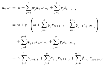 (A1)
(A1) . Therefore, we have
 (A2)
(A2)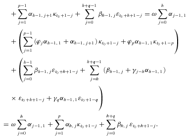 (A3)
(A3)Consequently, it is also valid for the case of n = h. This completes the proof. Q.E.D.
APPENDIX B
 , to ease the complexity of the derivation. If we sum Equation (6) for n = 0, …, N – 1, we obtain
 (B1)
(B1)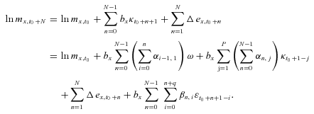 (B2)
(B2) , for j = 1, …, p, are known because the historical data of mortality indexes conditional on
  are available. The last term in the right-hand side of Equation (B2) can be rewritten as follows:
 (B3)
(B3) is defined as in Equation (11). Thus, the mortality force at age x during calendar year t0 + N takes the form:
 (B4)
(B4) is known at time t. This completes the derivation of Equation (7). Q.E.D.
APPENDIX C
 , the mean of
  is given by
 (C1)
(C1) can be expressed as
 (C2)
(C2)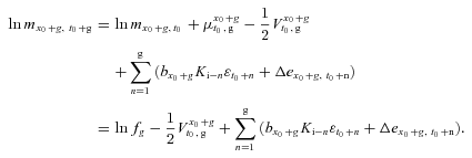 (C3)
(C3) (C4)
(C4) , conditional on
  , follows a normal distribution with 0 mean and variance
  , we obtain
 (C5)
(C5)Substituting Equation (C5) into Equation (C2), we can obtain the second moment of  . This completes the proof of Proposition 2.Q.E.D.
APPENDIX D
 (D1)
(D1) is the gamma function, which has the property
  . If a random variable Y is reciprocal gamma distributed, its inverse, 1/Y, is gamma distributed. We can show, using standard calculus techniques, that
 (D2)
(D2) (D3)
(D3)In view of Equation (13), An represents the arithmetic sum of the mortality rates, which makes the valuation of the survivor swaps and survivor floors more complicated, because An is not lognormally distributed. A common approach to this problem has been to approximate the state-price density of An using a lognormal function with various moment-matching techniques (Huynh, 1994). Milevsky and Posner (1998a, 1998b) demonstrate that in the pricing of Asian options, the sum of the correlated lognormal random variable is closely approximated by (and converges at the limit to) the reciprocal gamma distribution; in pricing basket options though, the reciprocal gamma approximation is better than the lognormal approximation and very accurate compared to a Monte Carlo simulation. Consequently, we use the reciprocal gamma distribution proposed by Milevsky and Posner (1998a, 1998b) as an approximation of the state-price density of An.
 and refer to it as
  . To moment match to a reciprocal gamma distribution, we find the parameters
  and
and  of
of  in terms of the first two moments. From Equation (D2),
 (D4)
(D4) and
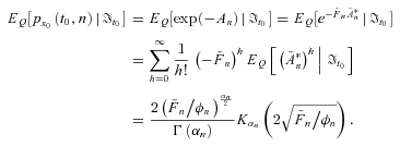
and  . Therefore, in view of Equation (D3), the expectation of survival probability
  is given by
 (D5)
(D5)This completes the proof of Equation (29). Q.E.D.
APPENDIX E
 and
and  , we recognize
 (E1)
(E1) is the probability density function of the reciprocal gamma distribution, which satisfies
 (E2)
(E2)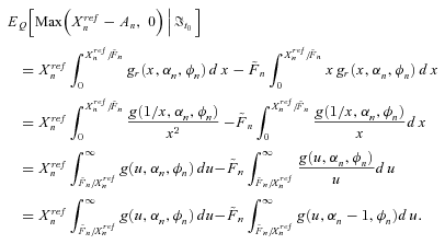 (E3)
(E3) and
and
 (E4)
(E4) (E5)
(E5)
REFERENCES
 , where LLF is the log-likelihood and NPS is the effective number of parameters being estimated.
 .
.


