Managing Systematic Mortality Risk With Group Self-Pooling and Annuitization Schemes
ABSTRACT
Group self-annuitization (GSA) schemes are designed to share uncertain future mortality experience including systematic improvements. Challenges for designing group pooled schemes include decreasing average payments when mortality improves significantly, decreasing numbers in the pool at older ages, and the impact of dependence from systematic mortality improvements across different ages of members in the pool. This article uses a multiple-factor stochastic mortality model in a simulation study to show how pooling can be made more effective and to quantify the limitations of these pooling schemes arising from the impact of systematic longevity risk.
INTRODUCTION
Internationally there has been a significant shift to defined contribution schemes to fund retirement and a reduction in pension funds providing longevity protection post retirement. Increasingly, attention has been turned to the postretirement phase and financial arrangements to convert accumulated lump sums into retirement incomes. These policy issues are well covered in recent World Bank discussion papers (Rocha and Vittas, 2010; Vittas et al., 2010). The ideal post retirement income provides consumption income with both longevity insurance and inflation indexation. Yaari (1965) demonstrates the welfare benefits of ordinary life annuities because of the longevity insurance protection provided under a standard life-cycle consumption model with perfect markets, actuarially fair annuities with no loadings and rational individuals with no bequest motives. Davidoff et al. (2005) show that there are benefits from some level of annuitization under more general assumptions. Although annuity prices are not actuarially fair, risk-averse individuals will still value annuities (Mitchell, 2001). Stevens (2010), among others, includes analysis of annuity decisions showing how systematic mortality risk reduces the attractiveness of life annuities.
There are many reasons advanced as to why there is a lack of well-developed annuities markets despite the potential longevity risk benefits. From a demand perspective, these include lack of liquidity, bequest motives, poor value for money, and availability of public pensions (Friedman and Warshawsky, 1990; Hurd, 1989; Mitchell et al., 1999). From the supply perspective, insurers incur significant capital costs in guaranteeing lifetime incomes because of the significant uncertainty of individual longevity prospects. Adverse selection and lack of underwriting in the life annuity market also leads to significant costs for suppliers of life annuities. Evans and Sherris (2010) review demand and supply factors in developing a life annuity market in Australia.
An approach to the management of uncertain future longevity, presented in Piggott, Valdez, and Detzel (2005), is referred to as group self-annuitization (GSA), which is designed to pool idiosyncratic risk with individuals bearing systematic risk. Individuals invest into the pool and are paid an annuity income that varies with the realized mortality experience. As individuals exit the pool from death, their remaining capital is shared among the survivors in the pool in the form of mortality credits. GSAs do not involve payment guarantees and do not require costly capital to support guarantees as compared to an ordinary annuity. They are designed to generate a retirement income similar to a life annuity. They are not designed as investment vehicles, as are variable annuities, so that investment risk including interest rate risk is minimized. Variable annuities are products designed to generate variable retirement income through exposure to investment markets. GSAs are not designed as variable annuities.
Valdez, Piggott, and Wang (2006) addressed adverse selection and demand issues for GSAs. Arrow (1969) provides an early discussion of the Pareto optimality of pooling differing risk types. Abel (1986) and Sinha (1989) consider adverse selection for ordinary annuity funds with known heterogeneous mortality probabilities. Valdez, Piggott, and Wang apply a similar utility framework to GSAs to show that annuitants will naturally adversely select against both conventional annuities and GSAs. The extent to which adverse selection is exercised against GSAs is lower than that of conventional annuities given certain utility function conditions.
Stamos (2008) extends Valdez, Piggott, and Wang (2006) by investigating the optimal consumption problem for fund participants in a portfolio choice framework. He shows that the expected mortality credit achieved by members who survived increased with the number of members in the pool. The expected optimal consumption as a proportion of initial wealth increased with the number of fund members. A similar pooling scheme is presented by Sabin (2010) known as Fair Tontine Annuity, or FTA, in which “fairness” is achieved by ensuring that pool members' expected benefits did not depend on the mortality experience of others in the pool.
Under existing sharing arrangements, as in Piggott, Valdez, and Detzel (2005), benefit payments can significantly decline over time, driven primarily by the improving trend of underlying human mortality. In addition, the volatility of benefit payments increases over time, arising from the uncertainty in mortality forecasts as well as the random deviation of experienced deaths from population mortality. This is especially the case at the older ages where numbers of survivors in the pool are smaller.
Group pooling will be more effective when individual benefit payments do not have a significant expected downward trend over time and future benefit payments do not have too high a level of volatility. Dependence between individual lives created by common drivers of mortality improvements has the potential to undermine pooling effectiveness, not only because of declining payments, but also because of systematic longevity risk that cannot be reduced with increases in pool size. Group pooling arrangements need to consider the extent that both of these factors can be managed in the pool.
This article assesses the effectiveness of GSA schemes allowing for systematic but uncertain longevity trends. A multifactor stochastic version of the Gompertz-Makeham (GoMa) model is used to capture both dependence across ages and systematic mortality improvements over time. The model is fitted to historical data for Australian males. Other developed countries mortality experience has been similar to Australia and so the results are broadly applicable. Simulation is used to quantify the extent to which benefit payments will decline over time, due to the inability of GSA benefit payment calculation rules to capture systematic mortality improvements. The extent to which the volatility of benefit payments increases over time is also quantified using the model. GSAs with a single cohort can only pool nonsystematic risk. Introducing other cohorts of the same initial age makes it practical to pool systematic risk across cohorts.
An aim of a GSA is to generate relatively smooth annuity payments in the pool. The investment of the GSA pooled funds needs to match the expected future cash flows. The interest rate risk associated with uncertain future improvement in mortality can be managed with a dynamic immunization strategy. Longevity hedging instruments such as longevity bonds can also reduce the cash flow mismatch risk. The investment management of interest rate risk in a GSA pool is less critical than for a guaranteed annuity because there are no guaranteed payments. However, interest rate risk can be effectively managed for annuity products when mortality is uncertain with systematic improvements as discussed in Tsai and Wang (2011) and Ngai and Sherris (2011). Uncertainty in real interest rates is included to quantify the impact of interest rate risk.
The extent to which these pooling arrangements can be made effective is a main aim of this article. Current pooling arrangements include new annuity factors based on the mortality experience as it is realized. GSA benefit payments will decline at the older ages with this approach. A method is proposed to share systematic mortality improvements in a GSA arrangement so that they are pooled and borne by the collective rather than the individual, extending and generalizing pooling arrangements in Piggott, Valdez, and Detzel (2005). By including the systematic trend of future mortality improvements in the calculation of annuity factors for benefit payments, the expected decline over time is significantly reduced. Pooling effectiveness is assessed both with and without expected future mortality improvements.
The article is organized as follows. The first section discusses the technical specifications for GSA pooling. The second section discusses the mortality model and the third section outlines the GSA fund value simulation procedures. Results of the analysis are presented and discussed in the fourth section, including the improvements to pooling methodology covered in this article. Finally, the main findings of this article are summarized in the fifth section.
ANALYSIS OF GSA SCHEMES
The analysis of GSA schemes follows that in Piggott et al. (2005). A generalization of their procedure is presented here and explained.
Benefit Payments
 (1)
(1) denotes the total fund value of all surviving members at time t and
  denotes the fund value of individual i conditional on survival. The * superscript denotes survival to time t.
Payments are adjusted over the time period t with an interest rate factor, where R is the expected interest rate and Rt is the realized interest rate, a mortality adjustment factor (MEA) and a separate changed expectation factor (CEA) to allow for changes in experienced mortality and in future expected mortality.
 and an initial payment is determined based on

The annual effective nominal interest rate, expected and realized, used throughout this article is 5 percent, equivalent to a force of interest of δ = 0.048790164, which is the approximate level of current long-term government bond yields in Australia.

 , denotes the inherited amount of fund balance given survival after the remaining wealth of deaths of pool members is distributed to those who survive, at time t.
Modification of Pooling Benefit Calculation
In Piggott, Valdez, and Detzel (2005), the MEA is separate from the CEA. The mortality adjustment factor allows for deviation from the expected number of deaths experienced by a GSA fund, whereas the changed expectation adjustment allows for a permanent shock to the underlying mortality. These two effects are difficult to differentiate between. For example, if additional deaths were experienced in a GSA they could either be the random deviation away from the expectation or they could be the result of a permanent increase of the underlying mortality rates. These two adjustment factors are incorporated into a single factor in this article. Initially the adjustment factor will not include expected future mortality improvements. Later, these will be included to show the importance of this in the pooling.
The mortality model is used to determine annuity factors. As the underlying rate of mortality evolves and the survival probabilities, px, change, these will be represented by px,t where t is the time that the survival probabilities apply. The actuarial annuity factor  changes every year, as the new mortality rates are revealed and an updated current life table is generated. These annuity factors will be denoted as
  , representing the actuarial present value of a $1 life annuity for a life aged x, calculated at time t, using all available mortality information at that point in time. These factors do not include expected future mortality rates. They are based on the updated dynamic life table generated by the mortality model at the current time.


 (2)
(2)The calculations are performed at time t based on mortality information at time t.

 (3)
(3)This relationship defines the fund balance after investment accumulation but before any inheritance from mortality credits from deaths. For the fund as a whole,  because the fund balance is always preserved. The relationship between
  (the survived fund balanced before inheritance) and
  (after inheritance) reflects the mortality experience sharing.

 is the total adjustment factor. It is important to note that
  is not
  , as in the Piggott et al. (2005) sharing arrangement. They have

 is dependent on the cohort to which it is being applied. This requires a subjective judgment as to how to translate the realized survival experience into a cohort-specific permanent improvement factor CEA dependent on cohort, and a universal volatility factor MEA independent of cohort. The exact way in which this can be done is subjective. A single factor
  universal across cohorts avoids this ambiguity in the sharing rules.
The approach shares systematic mortality risk experience across cohorts. Sharing arrangements are always conflicted in balancing solidarity for the whole pool and actuarial fairness for individuals in the pool. By sharing systematic risk across cohorts, provided each cohort is made better off in terms of benefit payments or benefit volatility, sharing rules are beneficial to all cohorts. Because the age of the cohorts is still used in the sharing rules at an individual level, allowance for cohort idiosyncratic mortality experience is also pooled.
 (4)
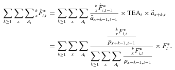
(4) is derived using Equation (3), and the benefit payment amount is then subsequently calculated using Equation (2). This expression has a simple interpretation. The fund value inherited by an individual is simply a weighted portion of the total available fund value. The weight is determined by the combination of
-
 , the fund value of the individual before inheritance, and
 - px+ k−1,t−1, the expected survival probability of the individual for the previous calendar year.
MORTALITY MODEL
There are many stochastic models for mortality that have been developed and applied to life insurance including those in Dahl (2004), Cairns, Blake, and Dowd (2006), and Milevsky and Promislow (2001). The mortality model adopted to demonstrate the impact of systematic risk on GSA benefit payments is a stochastic dynamic GoMa model similar to the Gaussian Makeham model in Schrager (2006).
 (5)
(5) (6)
(6) (7)
(7) (8)
(8) (9)
(9)The model allows for systematic improvements in mortality and captures dependence in mortality changes across ages. Dependence in the factors across ages is captured by the standard correlation coefficient. The model formulation allows the derivation of closed-form survival probabilities and approximate annuity factors, which suits the simulation computations (Schrager, 2006; Milevsky, 2006).


 .
.Long-term mortality improvements arise from negative parameter values for a1 and a2, whereas a deterioration would be represented by positive estimates for a1 and a2.
The model is fitted to data from the Human Mortality Database (2010) for Australian deaths and population data from the years 1965 to 2007. Male data for ages 60–99 are selected because GSAs are designed for retired individuals. Older ages are not included in fitting the model because of smaller number of deaths at these ages. Data before 1965 were omitted due to data collection limitations by the HMD before that year. This results in the data being reduced to incorporate 40 different ages across 43 years for a total of 1,720 observations.
 (10)
(10) , denotes a data value and a tilde,
  , denotes an estimated value.
Under standard Poisson deaths assumptions, with a central population exposure of  individuals in the pool aged x at time t have a death rate of
  . The conditional death rate
  has a mean of μx,t and variance
  . This is approximately normally distributed from the central limit theorem (CLT), so that
  .
.
To fit the model parameters to the data, the unconditional distribution of deaths,  , is required. This is determined by integrating the distribution function of
  with the distribution of μx,t. Although the unconditional distribution should be a normal distribution, closed-form analytical results do not exist if both the mean and variance in the distribution of
  are functions of μx,t, and hence, random.
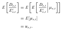

The approximation replaces the population parameters with sample estimates.
The volatility of the observed number of deaths varies with age. Even if the underlying variability of the true rate of mortality for a particular age was zero, the observed deaths data exhibit variability from the random date of death.

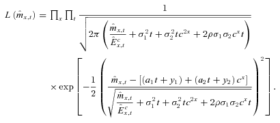
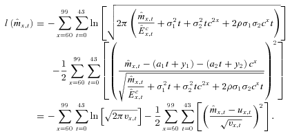 (11)
(11)The fitted parameters from the data for Australian males aged 65–99 for the period 1965–2007 for the GoMa mortality model, with time zero as the year of 1965, are given in Table 1.
| Parameter | Estimate |
|---|---|
 |
0.000322448 |
 |
0.000058809 |
 |
1.096559466 |
 |
−1.144811496× 10⁻¹⁰ |
 |
−3.832494756× 10⁻⁷ |
 |
3.639275565× 10⁻¹⁹ |
 |
1.145473323× 10⁻¹¹ |
 |
0.929491793 |

 , where p is the number of parameters estimated for significance level α percent. The Pearson's chi-squared test statistic is

 2, the null hypothesis is not rejected.
Mortality Model Assumptions
The GoMa model generally fits older age mortality period rates well and explicitly produces survival probabilities that are double exponential. Survival distributions are extreme value distributions allowing for analytical approximations and survival curves consistent with empirical data. Closed-form analytical expressions for survival probabilities and annuity factors are an advantage of the GoMa model if the survival probabilities are known. When the survival probabilities are simulated for future years it is only the current survival curve that is known. In this case, simulation is required to generate the future survival curves.
The Gaussian assumption in the model has the potential to produce negative mortality rates, which is an issue with any Gaussian model. Schrager (2006) suggests that parameter values can be estimated to reduce the probability of negative rates. For a mean-reverting model the possibility of negative mortality rates will be small. However for a non-mean-reverting model as adopted here, a modification is required to eliminate the possibility of negative mortality rates.
The model simulations exclude negative mortality rate paths. The negative scenarios are replaced with simulations that do not have negative mortality rates.
Mortality models that have lower age dependence will produce benefit payments that show greater advantages from pooling across cohorts, due to reduced levels of dependence. Alternative mortality models with systematic mortality improvements will produce qualitatively similar results.
The GoMa model does not model cohort improvements explicitly and allows for these only through the relative changes in the two factors Y1 and Y2, which are positively, but not perfectly, correlated. Expected trends in future mortality rates differ across cohorts.
The model is estimated using population mortality, which ignores the impact of any differences between a particular GSA pool and the population. This is used to estimate the mean and volatility of individual mortality rates. Because population data were used for the models, estimates sampling variability are small and produce relatively accurate estimates of the individual mortality rate parameters.
Impact of Mortality Improvements and Systematic Risk
Individuals in a GSA pool have both idiosyncratic and systematic longevity risk. The idiosyncratic risk is the risk that is reduced most by pooling. These risks are independent across individuals in the pool. Increasing the pool size reduces the idiosyncratic risk as measured by the variability in the average survival time in the pool. The variability of payments is also reduced by pooling because payments vary with the idiosyncratic risk of the pool.
Systematic risk arises from dependent risk factors that impact the survival probabilities of all individuals in the pool to a greater or lesser extent. High levels of systematic risk reduce the effectiveness of pooling compared to a situation with only idiosyncratic risk. Larger pools and pooling across multiple cohorts reduces the volatility of benefit payments arising from idiosyncratic mortality risk to individuals at older ages. Pooling the longevity risk allows higher benefit payments to be made for any given probability of exhausting the pool funds than for the case of an individual self-insuring longevity risk by drawing down savings so as to have the same chance of exhausting their savings.
- The existence of systematic mortality improvements from the dependence between lives and
- The long-tailed distribution for aggregate survival distributions, as reflected by the GoMa model, where there is a downside skewed tail.
Systematic risk is borne by the fund members in a GSA pool. This alleviates the need for capital. However, systematic risk undermines effective pooling because of the higher volatility in payments and declining benefit payments with expected future improvements. Volatility in payments can be pooled across different cohorts to reduce overall volatility.
The pooling is made more effective by allowing for future expected improvements based on the mortality model. The model evolves mortality rates randomly through time with both expected changes and variability around those changes. At any future time, it provides expected future mortality rates. The uncertainty in the mortality model arises from the random time t evolution of the factors Y1 and Y2. At any future time, given the values of these factors a survival curve can be constructed based only on past mortality information.
 (12)
(12)Expected future survival probabilities take these expected improvements in the model mortality rates into account. An approximation is used for convenient computation of annuity values; otherwise, extensive simulations are required for computing future survival rates and values of life annuities.
 (13)
(13)

 denotes the updated actuarial present value annuity factor, taking into account expected systematic mortality improvements, where there are long-term expected mortality improvements,
  .
.The benefits in the GSA risk pool are then computed based on expected future mortality rates at t and current information about mortality after including the sharing of mortality credits from the deaths in the pool. A new projected expected survival rates life table is generated for each t, resulting in a new  for each x that takes into account future expected mortality improvements based on the mortality model.
This approach incorporates mortality expectations dynamically without the need to measure changes in mortality against an assumed future experience. The annuity factors  and E[px+ s,t+ s |μx,t] are computed numerically.
Benefit payments are then determined by Equation (2), using the annuity factors to account for improving mortality. By using  , and hence increasing
  at all ages, benefit payments at entry will be lower but will be closer to level at future times.
Mortality Projections

 (14)
(14)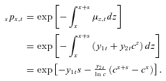 (15)
(15)This rate is evaluated at time t, where information about the future has not yet been revealed. These survival probabilities do not take into account future mortality evolution, because this is unknown at point t in time. This closed-form solution is a computational advantage in the use of a GoMa mortality model.
 (16)
(16)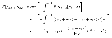 (17)
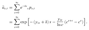
(17)These computations are made for every year for use in Equation (2) to arrive at individual benefit payments for both the case where only current mortality information is used in the annuity factors and the case where expected future mortality is included.
SIMULATION METHODOLOGY
- Future mortality rates are forecasted by simulation of the random dependent factors Y1t and Y2t driving mortality changes.
- These are bivariate normal simulations.
- A mortality matrix x age by t time is generated.
- Simulations with negative rates are replaced with paths with positive rates.
- Determine survival probabilities from the simulated mortality rates.
- Probability of survival for an individual in a particular year is determined using Equation (15) and setting s = 1, for each year. This is then repeated every year for all fund members, for their corresponding ages x for each time t in the fund.
- Determine the actuarial present value annuity factor using Equation (16) for every year, and every member, for their corresponding ages x at time t in the fund.
- Simulate the death and survival of fund members every year with a
 random variable, where 1 denotes survival and 0 denotes death. Death events are doubly random, where the deaths are random, and the survival probabilities px,t are also random, driven by random underlying mortality rate simulations.
 - Determine the inherited fund balance from the deaths and benefit payment for each of the survived fund members at the beginning of every year, using the algorithm in Equations (2) to (4).
This procedure produces one complete simulation for all the fund members. This process is repeated so that many simulations are generated, and the resulting benefit payment amounts are summarized in a distribution for differing future times (and ages). Because the random parameters, or factors, in the model impact all ages there is systematic risk across individuals. For individuals of the same age the future mortality shocks are also treated as common to individuals of the same age.
- A starting contribution value of $100 (benefit payments as a percentage of the starting contribution are unchanged by differing starting contributions);
- A time horizon of 40 years (so the oldest age included is 105);
- All pools start at time 0, which is the year of 2007 for the mortality model;
- The mortality rates for time zero are known; this provides approximately $8.99 in benefit payments, computed by
 to 65-year-old males at time 0 (not including expected mortality improvements);
 - Initial entry age of participants is 65 unless stated otherwise;
- All fund members are males because the mortality data used for calibration of the model were Australian males; and
- An annual effective rate of interest of 5 percent, which equates to a constant force of interest of δ = 0.04879016. In all simulations the realized interest rate return is the same as the expected rate of interest.
RESULTS AND DISCUSSION
The impact of pool size on future benefits is assessed by deriving the distributions of benefit payments at future times (and ages). The cases considered include with and without the method proposed in the article to enhance the effectiveness of pooling systematic risk. The impact of admitting new entrants to the pool is also assessed by considering the distribution of future pool payments and the impact on volatility of payments at different ages. The cases with and without allowance for expected future mortality improvements are shown. The impact of inflation on benefits payments is also considered. To illustrate the impact of stochastic interest rates, a case with a stochastic real rate of return calibrated to Australian data is also provided.
Presentation of Results
Benefit payments to individuals are illustrated by showing the  percentile, median, and
  percentile of the simulated outcomes at each age over future years. These distributions clearly illustrate the variability of future payments. The measures show the level of benefit payment that pool payments will fall below (
 percentile) 5 percent of the time and increase above (
 percentile) 5 percent of the time. The median is the payment value with an equal likelihood of being either above or below. These measures reflect those recommended in the Review into the Governance, Efficiency, Structure, and Operation of Australia's Superannuation System completed under Cooper (2010).
 percentile are given by the

This article has used 5,000 simulations for scenarios, unless specified otherwise, because the CIs demonstrate this is sufficient to produce reliable simulation estimates.
All graphical results are presented in a comparative format with identical axes. 95 percent CIs have been plotted. All benefit payments are for the surviving pool individuals and conditional on a pool member surviving.
Self-Insurance: Single Cohort, Single Individual
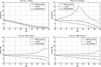
For an individual who self-insures longevity risk, the benefit payment distribution under existing GSA rules is displayed in the top left panel of Figure 1 for a single individual aged 65 entering the pool at t = 0. For self-insurance, there are no mortality credits from other members in the pool and the mortality improvements result in declining payments throughout the individual's life. The original annuity factor used for the GSA assumes an average lifetime based on a large pool of independent individuals. As individuals survive to older ages the chart shows the clear impact of systematic longevity risk. Too much is consumed too early because survival can occur past the average lifetime reflected in the annuity factor at time t = 0. There is not much variability because there is only one member and experience is fully allowed for in the annuity factors.
Increasing Pool Size and Pooling Benefits
Figure 1 also shows the distribution of payments as the pool size is increased to 10 (top right panel), 1,000 (bottom left panel), and 10,000 (bottom right panel). For smaller pool sizes the variation in the benefit payments at future ages is very wide and the upside for higher benefit payments increases early on. For scenarios where mortality deteriorates with a small group in the pool, the survivors benefit from larger mortality credits early on. However, as the pool size diminishes through time the mortality credits reduce. This is referred to as a “lucky hump” or “ontine effect” for small pools. The tontine benefit arises for survivors in small pools where there is a higher probability of deaths occurring that represent a given proportion of the pool.
As the pool size increases, this tontine effect, which occurs only when the survivor pool is small, is much reduced and occurs at later ages. Benefits are higher for longer than in the self-insurance case because of the pooling effect of mortality risk. With 1,000 initial members in the pool, which would normally be sufficient to benefit from risk pooling with only idiosyncratic risk, the upside tontine effect remains significant at the older ages. With 10,000 initial members in the pool the effect is much reduced, but the wide range of benefit outcomes at the older ages remains, along with the reduction in average benefits. With no allowance for future expected mortality improvement benefits drop for the older aged survivors in the pool.
With a single cohort in the pool, even with significant sized pools, there are a number of factors that clearly undermine the effectiveness of GSA. One is the decline in benefits at the older ages reflecting the impact of systematic improvement in mortality. The other is the widening range, and increasing volatility, of future benefits in the pool. The extent of the downside is of particular concern because the 5 percent worse cases at the older ages represents a significant reduction in benefit payments.
To provide a numerical comparison of these effects at the older ages, Table 2 shows the 95 percent CIs for the three percentile estimates for the amount of benefits received by a single individual at t = 25, when he is aged 90. The benefits of risk pooling can be seen for GSA in terms of improvements over self-insurance along with the limitations.
| Pool size |  Percentile Percentile |
Median |  Percentile Percentile |
|---|---|---|---|
| 1 | (1.24,1.27) | (2.00,2.03) | (3.09,3.14) |
| 10 | (3.69,3.79) | (7.50,7.70) | (19.58,20.19) |
| 1,000 | (5.49,5.77) | (8.18,8.33) | (10.81,11.15) |
| 10,000 | (5.50,5.86) | (8.27,8.47) | (10.62,10.83) |
Results With No Allowance for Future Expected Mortality Improvements
- Increasing the pool size will increase the median and the 5th percentile of benefit payments for GSA members. It will also decrease the absolute volatility of the payments.
- As the number of members in the pool increases, it becomes more difficult for further pooling benefits to be realized. Most of the significant pooling benefits are realized when the pool size reaches 1,000.
- The volatility of benefit payments at old ages, is far greater than those at younger ages, reflecting the impact of systematic longevity risk and reducing pool size.
- The median and
 percentile values of payments decline over time regardless of the number of people in the pool. This occurs because of the expected improvement in mortality. Approaches to GSA benefit determination that do not include this will result in payments being too high early on. Smaller pool sizes at older ages result in higher reductions.
 - The
 percentile increases first before declining, due to the tontine effect in small pools. There is always a small chance that a sizable proportion of people will die early, and this increases for small pool sizes. For the members who are lucky enough to survive, they benefit from those who died, leaving them with substantially larger benefit payments. Eventually, the benefit payments decline regardless of the tontine effect.
 - As the pool size increases, the tontine effect is deferred to later, as the actual deaths are closer to the deaths expected.
- The absolute volatility of payments is large even allowing for increasing pool size.
Pooling With New Cohorts
Piggott, Valdez and Detzel (2005) proposed pooling multiple cohorts in the same pool. This has to be carefully considered because it will be favorable for the 65-year-old cohorts to pool with older cohorts entering the pool at the same time unless pooled benefit payments are determined separately for cohorts of different age at entry to the pool. The benefits of risk pooling would otherwise be diminished and older cohorts would be less willing to participate.
Effective risk pooling arrangements with intergenerational solidarity are possible if members of older cohorts share experience with younger cohorts, where all the cohorts enter the pool at the same age. New cohorts of 65-year-olds would continuously join existing pools in subsequent years. The benefits are that improvements, or adverse mortality changes, at the older ages would be shared across all ages, resulting in a more level benefit payment across ages of the members in the pool. Also, the volatility at the higher ages would be shared with the lower volatility at the younger ages, resulting in increased chance of adequate benefits at the older ages.
To quantify the benefits of such a pooling arrangement with new entrants at the same age, a scenario with new members entering every year at age 65 is considered, and this is compared with scenarios where new members aged 65 enter every 5 years. For each of the scenarios, one thousand members entering aged 65 enter at time 0 are pooled with the survivors of the cohorts of the thousand 65-year-olds who entered at earlier times.
The results of these dynamic pooling arrangements are shown in Figure 2. Table 3 shows the 95 percent CIs for the three percentile estimates for the amount of benefits received by a single individual at t = 25, when he is aged 90, under the dynamic pooling arrangements, with dynamic pooling occurring every year (left panel) and every 5 years (right panel).

| Dynamic Pooling Frequency |  Percentile Percentile |
Median |  Percentile Percentile |
|---|---|---|---|
| Every year | (5.47,5.78) | (8.26,8.47) | (11.11,11.39) |
| Every 5 years | (5.66,5.88) | (8.31,8.41) | (10.67,10.84) |
| Never | (5.49,5.77) | (8.18,8.33) | (10.81,11.15) |
Dynamic pooling also reduces the volatility of benefit payments of older members significantly. This occurs because the idiosyncratic volatility of deaths experienced in the pool will diminish when younger cohorts are allowed to enter. Annuity factors for pooling and benefit payments explicitly allow for the age of members in the pool. The size of the pool is more stable over time and the higher volatility of older ages is shared with lower volatility at younger ages in the pool. Dynamic pooling every 5 years does not produce significantly different results from pooling new cohorts every year.
Dynamic pooling where individuals from other cohorts join existing funds on a frequent basis will reduce the high volatility of benefit payments experienced by people surviving to old ages. These benefits will be available to all those entering the pool if they survive to old ages and new entrants are admitted to the pool at the same entry age on a regular basis.
Dynamic Pooling With Future Expected Improvements
The pooling results so far use an annuity factor based on the simulated mortality experience as it evolves without explicit allowance for future expected improvement. By using an updated  factor, future benefit payments are less susceptible to reductions from systematic mortality improvements, and the equity of pooling arrangements between different cohorts is improved. To demonstrate the impact of this assumption, a group of one thousand 65-year-olds are assumed to enter the pool at t = 0, with subsequent groups of one thousand 65-year-olds entering the same pool every 5 years. Benefit payments are determined based on the updated
  factor, taking into account expected mortality improvements.
The benefit payment distribution is displayed in Figure 3 and Table 4. Table 4 presents the benefit payment received by a pool member when he is 70 years of age at t = 5, 80 years of age at t = 15, and 90 years of age at t = 25.

 Factor with Systematic Allowance Used to Calculate Benefit Payments
| Age |  Percentile Percentile |
Median |  Percentile Percentile |
|---|---|---|---|
| 70 | (7.78134,7.84896) | (8.76987,8.81321) | (9.64436,9.70525) |
| 80 | (6.84956,7.06950) | (8.89730,8.97150) | (10.57074,10.67242) |
| 90 | (5.94495,6.28521) | (9.10051,9.24033) | (11.57233,11.73409) |
By allowing for systematic mortality improvements in the determination of the actuarial present value annuity factor, the amount of benefit payments received by individuals shows much reduced declines over time.
The updating of the annuity factor for determining benefit payments of surviving members in the pool to include expected improvements has largely offset the reduction in median payments. The systematic nature of mortality changes means that absolute volatility will increase through time regardless of the risk sharing rules in the pool. Mortality uncertainty increases over time and impacts older ages more significantly than younger ages.
At the older ages there is always a declining trend in benefit payments affecting the median and the  percentile of outcomes. The survival distribution for the GoMa model is an extreme value distribution, and with systematic mortality improvement the pooled distribution has extreme value properties so that the distribution has a significant skew to the downside at the older ages.
Nominal Payments
The payments in the results have been standardized to an initial amount of $100. The absolute level of payments is readily determined. Consider as an example a male individual earning on average $70,000 per year in salary from age 25 with an average investment return rate over 40 years of 5 percent. This male individual will accumulate  = $761,038, which is the contribution times the actuarial accumulation factor for 40 years, in retirement savings by the age of 65 under a 9 percent contribution. This is the contribution rate for the Australian compulsory SG scheme.
In a pool with one thousand 65-year-olds entering the fund every 5 years, and where the annuity factor takes into account expected mortality improvements, the corresponding benefit payments based on Figure 3 and Table 4 for an initial contribution to the GSA of $761,038 are shown in Table 5. Tables with other initial contribution amounts can be readily constructed.
 Factor With Systematic Allowance Used to Calculate Benefit Payments, and Where the Initial Contribution Is $761,000
| Age | 5th Percentile | Median | 95th Percentile |
|---|---|---|---|
| 70 | (59215.98,59730.61) | (66738.72,67068.57) | (73393.57,73856.99) |
| 80 | (52125.14,53798.93) | (67708.46,68273.09) | (80443.35,81217.13) |
| 90 | (45241.09,47830.43) | (69254.85,70318.9) | (88065.41,89296.42) |
This male will receive around $68,000 annually from a GSA fund on the balance of probabilities (reflected by the median) should he choose to participate in such a fund with the entire amount of his retirement savings.
In such a GSA fund, there will be a 5 percent probability that he will receive less than around $45,000 annually in his retirement, an amount that would still be adequate as a retirement income. GSAs, implemented as discussed in this article, will provide a sustainable and feasible retirement product for retirees, even after allowing for adverse outcomes.
Substantial pooling benefits are gained when the pool size reaches around 1,000. The Australian Bureau of Statistics reported that there were 97,708 Australian males turning 65 in 2009. A hypothetical major retail GSA fund with a market share of 10 percent of Australian males at age 65, would have approximately 10,000 members. One thousand members would represent a relatively small fund. The major issue for such small funds is the expense of managing the fund. However, the methodology for managing a GSA is efficient to implement, and smaller funds may be viable, especially if the technology is available in a standard adminstration system.
Indexed Benefit Payments and Random Real Interest Rates
Interest rate risk for annuity products including GSAs is managed using immunization strategies. Retirees desire benefit payments that are inflation indexed, such that their income does not diminish in purchasing power over time. Without indexed bonds or longevity bonds, real returns will be uncertain. The risk of random real returns is an important factor along with longevity improvements in assessing GSA pooling.
To consider the impact of uncertain real rates of return on inflation indexed payments, simulations were carried out with a stochastic real rate of return. Simulations with 5-year dynamic pooling and a pool size of 1,000 were carried out with stochastic real interest rates. In this case, investments are effectively assumed to be made in real return instruments with low volatility. The real rate assumed was the long-run historical average real interest rate for Australia from 1991, or 2.72 percent per annum. Uncertainty in the real rate of interest was modeled with a Cox–Ingersoll–Ross (CIR) stochastic real interest rate model, with a volatility factor of 0.0709, consistent with historical observations. The results are shown in Figure 4.

In real terms the adverse payment scenarios are roughly constant when increased by inflation. By including real interest rate uncertainty, the range for the upper and lower benefit amounts widens but not significantly. Systematic longevity risk remains the driving factor for volatility of payments.
CONCLUSIONS
The article extends and generalizes the pooling arrangements for GSAs as proposed by Piggott, Valdez, and Detzel (2005). The extent to which benefit payments decline over time and the extent to which the volatility of benefit payments increases over time have been mitigated through innovations in the risk pooling methodology. Under GSA pooling arrangements, benefit payments can be expected to decrease, and the volatility of payments expected to increase, over time.
This article has improved understanding of the implementation of GSA schemes and shown how the impact of systematic longevity risk can undermine their effectiveness. At the same time, strategies for pooling to improve the performance of risk sharing in the schemes with the introduction of new cohorts at the same age through time are assessed.
Increasing the pool size was shown to increase the benefit payments for GSA members and to decrease the absolute volatility of the payments. Dynamic pooling, where individuals of the same age join existing funds on a frequent basis, was shown to reduce the high volatility of benefit payments experienced by pool members surviving to old ages and to limit the decline in benefits for older ages. Using annuity factors that take into account future expected mortality trends also ensures the amount of benefit payments received by pool members will remain relatively stable over time.
A multifactor stochastic version of the GoMa was used to project mortality rates. The model was calibrated to Australian male mortality. The model included systematic and idiosyncratic mortality risk and allows analytical computations to be used to improve efficiency of the determination of pool benefit payments. Simulation was used to demonstrate the performance of improved risk pooling arrangements. The results hold for more general mortality models.
There are many aspects of longevity risk pooling that this article did not aim to address. A viable GSA pooling scheme must formally allow for heterogeneity for individuals of the same age. An example is pooling males with females. Sharing arrangements will have to recognize different longevity prospects for females and males. This is readily incorporated in the framework presented here.
Reinsurance is a possible approach to managing the systematic risk in a GSA where younger members would have reduced benefit payments earlier on to purchase a guaranteed narrower band for future payments from an external reinsurer. Another alternative is an investment in longevity bonds with payments linked to population mortality providing an offset to the systematic mortality of members in the pool. If an inflation indexed life annuity bond (longevity) market was available for investment, then it would be possible to reduce the systematic mortality risk through the investment of the pool funds. The interaction between investments and mortality risk was not covered in detail in this article. An analysis of the hedging effect of such bonds on annuity payments is provided in Ngai and Sherris (2011).


