Loss Coverage as a Public Policy Objective for Risk Classification Schemes
The author can be contacted via e-mail: [email protected]
Abstract
This article suggests that from a public policy perspective, some degree of adverse selection may be desirable in some insurance markets. The article suggests that a public policymaker should consider the criterion of “loss coverage,” and that in some markets a policymaker may wish to regulate risk classification with a view to increasing loss coverage. Either too much or too little risk classification may reduce loss coverage. The concept is explored by means of examples and formulaic and graphical interpretations. An application to the UK life insurance market is considered.
Introduction
Much discussion of risk classification is concerned with the phenomenon of adverse selection or antiselection. The discussion is usually framed negatively: any degree of adverse selection is conceived as a problem that should be deprecated, avoided, or minimized. For many purposes, this perspective is useful. However, this perspective can be limiting if one is commenting on risk classification from a public policy viewpoint. Such comment often seems to retain the implicitly negative and deprecatory framing of adverse selection. This framing focuses on adverse selection as a possible obstacle to efficiency of contracting in insurance and implicitly assumes that promoting such efficiency should be the only or main focus of public policy. But from a public policy viewpoint, it is not clear that this exclusive focus is always appropriate, or that adverse selection is always adverse. From a public policy viewpoint, the restitution of some types of loss by insurance may be seen as a desirable objective, which policymakers often seek to promote (e.g., via tax relief on premiums). Some degree of adverse selection in some insurance markets may then be seen by a policymaker as desirable: it means that the right people, people more likely to suffer loss, will tend to buy (more) insurance. If the degree of adverse selection in an unregulated market is insufficient, a policymaker may wish to impose some restrictions on risk classification and so induce what has been called “regulatory adverse selection” (Polborn, Hoy, and Sadanand, 2006; Hoy, 2006). Some such restrictions are seen in many jurisdictions in practice.
The purposes of this article are to explore the idea that from a public policy perspective some degree of adverse selection may be desirable in some insurance markets, and to suggest the idea of loss coverage as a possible criterion for a desirable level of adverse selection. The remainder of this introduction outlines these ideas in general terms. The second section considers a simple example of how loss coverage may be increased by restrictions on risk classification and alternatively how it may not. The third section gives formulaic and graphical interpretations. The fourth section considers an application to the UK life insurance market. The final section gives conclusions and suggestions for further research. A more discursive treatment (but without the mathematical and graphical interpretations) was given in a recent review of risk classification (Thomas, 2007).
Throughout this article, I assume that the probability of a loss is independent of insurance coverage; that is, I ignore possible moral hazard. I also ignore the possibilities of government transfer payments toward higher risks or tax-and-subsidy schemes within the insurance market (Crocker and Snow, 1985) as remedies for perceived inequities arising from risk classification. I assume that all insurers are required to adopt similar risk classification regimes; that is, I ignore competition in risk classification of a “cream-skimming” nature. This assumption is not representative of extant markets with little or no regulation of risk classification, but in the context of policy restrictions on risk classification which are the focus of the article, it can easily be imposed by the policymaker. Finally, I assume that in all risk classification regimes insurers make zero profits in equilibrium.
While this article differs from much previous theoretical literature by suggesting that adverse selection can sometimes be beneficial, it follows the previous theoretical literature in assuming that adverse selection is a pervasive phenomenon and therefore worthy of theoretical attention. Empirical evidence on this point is somewhat mixed, perhaps partly because different researchers have placed different interpretations on testing for adverse selection. One simple interpretation is to test for positive correlation between the risk level and the amount of insurance purchased. Several studies along these lines have failed to detect the expected positive correlation for life insurance (Cawley and Philipson, 1999), auto insurance (Chiappori and Salanie, 2000; Dionne et al., 2001), and health insurance (Cardon and Hendel, 2001). On the other hand, “positive” test results for the presence of adverse selection have been reported for long-term care insurance (Finkelstein and McGarry, 2006) and annuity markets (Finkelstein and Poterba, 2004). These “positive” results tend to be based on demonstrating more subtle relationships between risk levels and behavior (e.g., chosen rate of increase and capital protection for annuities, private predictions of benefit utilization in long-term care) rather than simple correlations of risk and quantity purchased. However, the purpose of the present article is to suggest that if restrictions on risk classification increase adverse selection, this may not be a bad outcome from a public policy perspective. In this context, it is adequate to assume that restrictions on risk classification do tend to induce adverse selection.
The idea of increased loss coverage as a desirable outcome from a public policy perspective bears some resemblance to a result in a previous article (Cummins and Weiss, 1993) that presented a comparison of automobile insurance under alternative tort and no-fault regimes in terms of stochastic dominance theory. The first part of the article by Cummins and Weiss (1993) assumes that insurance is actuarially fair and that accident rates are the same under both tort and no-fault regimes; under these assumptions, Cummins and Weiss find that the no-fault regime is stochastically dominant provided the no-fault premium is higher than the tort premium, a result the authors describe as “seemingly counter-intuitive.” In the present article the analogous idea is that higher aggregate insurance premiums (equivalent to higher loss coverage) can be regarded as a desirable outcome.
Adverse to Whom?
To a noneconomist, the characterization of adverse selection might prompt the question adverse to whom? Most obviously, unanticipated adverse selection (i.e., adverse selection which is not allowed for in rating) may be adverse to an insurance company. Perhaps adverse selection is adverse to lower risks, who may pay more for insurance than they might otherwise have paid. In some models of insurance, adverse selection is also adverse in the sense that it implies reduced sales of insurance (although in the models developed later in this article, this is not necessarily the same as reduced coverage of losses). But it is not obvious that adverse selection is adverse to higher risks who obtain insurance they could not otherwise have obtained or pay a lower price than they would otherwise have paid. In many contexts, a policymaker might be particularly concerned that insurance should be available to higher risks. Some degree of adverse selection may then seem desirable—it means that the right people, people more likely to suffer loss, will tend to buy (more) insurance.
Loss Coverage
However, the question arises how much adverse selection is desirable? I suggest that in many markets, a reasonable objective for a public policymaker is to maximize the “overlap” of insurance coverages and loss events—the “loss coverage”—that is maximize the expected proportion of loss events in a population that is covered by insurance. This objective implies that the policymaker places higher priority on higher risk individuals being insured; for example, insurance of one higher risk individual is worth the same to the policymaker as insurance of two lower risk individuals if the probability of loss for each higher risk is twice that of each lower risk. In other words, insurances held by higher and lower risk individuals are regarded as equally desirable by the policymaker ex post, when all uncertainty about who will suffer a loss has been resolved, but insurances held by higher risk individuals are regarded as (risk proportionately) more desirable by the policymaker ex ante.
One way of maximizing loss coverage is to make insurance compulsory—either through social insurance or by laws that compel people to buy commercial insurance. For example, health care is provided through social insurance in many countries. Liability insurances that protect the interests of unidentified third parties or the public at large are often made compulsory. Employers' liability insurance and third-party motor insurance are examples of this in many countries in Europe. The losses compensated by these insurances are largely independent of the preferences and circumstances of the insured, and so compulsion is a well-targeted approach to achieving policymakers' desired (universal) loss coverage.
In some other types of insurance, such as life insurance, the policy motivations to increase loss coverage may be less compelling but are still present to some degree.1 However, in life insurance the need for and benefit from the insurance are directly affected by personal circumstances and preference of the insured. For example, a compulsory requirement for unmarried persons to purchase life insurance may often not increase loss coverage (because there is often no financial loss to a survivor if the unmarried person dies) and the cost of premiums to the single person may well be a negative benefit. One might exclude unmarried persons from compulsion, but of course some unmarried persons do need life insurance, and equally, some married persons do not. Overall, for insurances where personal circumstances and preferences are important, compulsion may be a poorly targeted and politically unpopular means of increasing loss coverage. It may be both more effective and more politically acceptable to leave purchasing decisions to individuals and attempt to increase loss coverage by other methods, such as targeting an appropriate level of adverse selection.
There may be a few insurance markets where there is little policy motivation to promote the restitution of losses through insurance. A clear example would be insurance against the cost of legal or regulatory penalties; a less clear example might be insurance of pet animals. In these cases, a policymaker would probably view loss coverage as a less important objective than in markets such as liability insurance, or health or life insurance. Indeed, the policymaker might even seek to minimize loss coverage, by discouraging the insurance. In extreme cases, this might mean banning the insurance. For example, the regulatory authorities in the UK prohibit financial firms from insuring against the cost of regulatory penalties, and insurance to provide chauffeur services after a drunk-driving conviction is prohibited in several jurisdictions.
Examples
The concept of adjusting the degree of risk classification to increase loss coverage is illustrated in the following model. There are two risk groups: a lower risk group with risk 1/100 and a higher risk group with risk 4/100. All insurance contracts are for a fixed sum assured. (This assumption allows adverse selection to be represented by varying proportional take-up of insurance in each of the two groups. It simplifies the presentation, but it is not necessary.) An individual's risk group is observable by the insurer. In Scenario 1 (shown in Table 1), actuarially fair premiums are charged to each risk group. In Scenario 2 (shown in Table 2), the insurer is not allowed to discriminate—there is a pooled premium rate irrespective of the risk group, and some adverse selection occurs. Take-up of insurance increases in the higher risk group and reduces in the lower risk group, and a slightly lower total number of policies are issued. The net effect is favorable, in that a larger proportion of the loss events is covered by insurance, that is the loss coverage is increased. In Scenario 3 (shown in Table 3), insurers are again not allowed to discriminate, but the adverse selection is more severe: coverage shifts further toward the higher risk group and the number of policies reduces more drastically. The net effect is unfavorable, in that the loss coverage is reduced.
| Risk Group | Lower Risk Group | Higher Risk Group |
|---|---|---|
| Population | 10,000 | 2,000 |
| Risk | 1/100 | 4/100 |
| Premium required | 1/100 | 4/100 |
| Take-up (members of group purchasing insurance) | 5,000 | 1,000 |
| (A) Expected loss events | 100 | 80 |
| (B) Loss events insured | 50 | 40 |
| Loss coverage: ΣB/ΣA | 0.50 |
- Notes on Scenario 1:
- (i) 50% take-up in both risk groups.
- (ii) 6,000 policies issued.
| Risk Group | Lower Risk Group | Higher Risk Group |
|---|---|---|
| Population | 10,000 | 2,000 |
| Risk | 1/100 | 4/100 |
| Premium required | 1.82/100 | |
| Take-up (members of group purchasing insurance) | 4,000 | 1,500 |
| (A) Expected loss events | 100 | 80 |
| (B) Loss events insured | 40 | 60 |
| Loss coverage: ΣB/ΣA | 0.56 |
- Notes on Scenario 2:
- (i) Some adverse selection.
- (ii) Take-up increased to 75% in the higher risk group.
- (iii) Take-up fallen to 40% take-up in lower risk group.
- (iv) Reduction to 5,500 in number of policies issued.
- (v) Higher loss coverage.
| Risk Group | Lower Risk Group | Higher Risk Group |
|---|---|---|
| Population | 10,000 | 2,000 |
| Risk | 1/100 | 4/100 |
| Premium required | 2.29/100 | |
| Take-up (members of group purchasing insurance) | 2,000 | 1,500 |
| (A) Expected loss events | 100 | 80 |
| (B) Loss events insured | 20 | 60 |
| Loss coverage: ΣB/ΣA | 0.44 |
- Notes on Scenario 3:
- (i) More adverse selection.
- (ii) 75% take-up in higher risk group (same as Scenario 2).
- (iii) 20% take-up in lower risk group (cf. 40% in Scenario 2).
- (iv) Reduction to 3,500 in number of policies issued (cf. 5,500 in Scenario 2).
- (v) Lower loss coverage than either of Scenario 1 or 2.
For some insurance markets, a public policymaker may regard Scenario 2, with higher overlap of insurance coverages and loss events, as superior to Scenario 1. That is, of these two scenarios, the case with higher adverse selection is superior. The more accurate risk classification in Scenario 1 produces a lower loss coverage.
Note that although slightly fewer policies are issued in Scenario 2 than in Scenario 1, more policies are bought by the right people, that is, people more likely to suffer loss. The loss coverage criterion captures the net effect of the shift in coverage toward higher risk lives (good) and the reduction in number of policies issued (bad).
On the loss coverage criterion, Scenario 3 is inferior to both Scenario 1 and Scenario 2. Although the take-up of insurance is higher in the higher risk group (good), this is more than offset by the reduction in take-up in the lower risk group (bad). The net result is that the loss coverage is reduced.
The essential difference between Scenarios 2 and 3 is the responsiveness of the lower and higher risk groups to changes in price. In these examples, the sizes of the lower and higher risk groups and their respective risks are fixed. More generally, the effect on the loss coverage of restricting risk classification will also depend on (1) the relative sizes of the lower and higher risk groups and (2) the relative risks of the lower and higher risk groups.


Note that the quantity (P2μ2/P1μ1) is the ratio of the total expected losses in the higher risk group relative to the lower risk group. Under the loss coverage criterion, the weight placed by the policymaker on proportional take-up in each risk group depends on the group's total expected losses.

Loss Coverage in Different Markets
The responsiveness of higher and lower risk groups to changes in price will probably be different in different insurance markets. This suggests that even if loss coverage were regarded as an equally important objective across different markets, different levels of risk classification may be socially optimal in different markets. It is difficult to say much about which markets: there are only a few data on price elasticities of demand for insurance (Pauly et al., 2003; Viswanathan et al., 2006) and no data that I know of on relative elasticities in higher and lower risk groups. Price elasticity would normally be expected to be lower in the lower risk group simply because of the lower price, but this need not mean that it is sufficiently lower. However, note that if the higher risk group tends to be declined altogether by insurers under unrestricted risk classification, we might expect a large increase in take-up—in effect, high price elasticity of (satisfied) demand—in that group when restrictions on risk classification are imposed.
Modified Definitions of Loss Coverage
In this article, loss coverage is defined as the proportion of loss events in a population that is covered by insurance. This is appropriate where the loss amount is the same for every event and the insurance coverage provides full restitution of the loss. In a more general setting where the loss amounts and insurance coverages are different for different insureds, loss coverage could be defined as the sum of losses covered/losses incurred over the whole population (both insureds and noninsureds). Alternatively, the view might be taken that the loss coverage objective should count only coverage of losses below some monetary limit for each insured, with excess losses disregarded,2 or alternatively, only coverage of some fraction of each insured's losses. It is easy to think of further possible definitions, but in this article “proportion of loss events covered” is used for ease of exposition.
Alternative Public Policy Objectives
Loss coverage is not suggested as the only criterion that a public policymaker should consider. In some markets, the role of accurate risk classification as an incentive to loss prevention may be a consideration; for example, this is often suggested for motor insurance, although a recent econometric study finds no evidence of such effects (Schwarze and Weim, 2005). In other markets, the policymaker might place a higher value on coverage of loss events in the higher risk group than in the lower risk group, perhaps because the former are seen as socially disadvantaged. The policymaker might also place value on ensuring the optional availability of insurance to members of the higher risk group, distinct from the actual take-up of the option. These approaches might be consistent with many other public policy initiatives directed at redressing disadvantages or social exclusion of the higher risk group. Nevertheless, while recognizing that alternative or additional policy objectives are possible, the concept of loss coverage provides a fresh way of thinking about the design of insurance systems from a public policy perspective. In many markets, loss coverage may be a useful criterion for an insurance-focused public policymaker.
Formulaic and Graphical Interpretation
In this section the demand for insurance di from population i is specified as a function of the premium charged, along the lines suggested by de Jong and Ferris (2006). The scenarios in the “Examples” section are reproduced and interpreted in terms of pairs of values of price elasticity parameters for the two populations.
A Functional Form for Demand

The formula can be interpreted as follows. When π is very small relative to μi demand from risk class i will be high. As the “premium loading”π/μi increases, demand from risk class i declines along an inverse exponential curve toward zero; this reflects the fact that if the premium loading π/μi is high enough, almost no one would buy insurance. When π=μi, the demand from risk class i is simply Piτi, that is, the number of members of risk class i times the proportion of members of risk class i who buy insurance at an actuarially fair premium. This specification allows a range of plausible demand curves to be specified for the relevant range of μ1 < π≤μ2.
The parameter τi, the fair-premium take-up of insurance for risk group i, reflects the fact that not everyone chooses to buy insurance at a fair premium. τ2 < 1 is required as a scaling factor to ensure that demand from the higher risk population does not exceed the total size of the higher risk population in the relevant range where the pooled premium is determined. In practice we might expect τ1 > τ2 because for lower risks insurance is cheaper relative to the prices of other goods and services, and life insurers who attempt to underwrite high risks report that the take-up on such quotations is often very low (de Ravin and Rump, 1996). For simplicity, we will set τ1=τ2= 0.5 through most of this article, except where specified otherwise, but this is not critical, and different values do not qualitatively change our results.3 The specification of τi as the proportion of members of population i who buy insurance assumes that all insurance is for unit sum assured; that is, every risk either buys one unit of insurance or none. This simplification is convenient for exposition, but it is not necessary; τi could alternatively be regarded as the fair-premium money demand for insurance from population i (as in de Jong and Ferris, 2006).

 and so the parameter λi is the price elasticity of demand for insurance when π=μi, that is, the “fair-premium elasticity.” It seems plausible that normally λ1 < λ2 because for lower risks insurance is cheaper relative to the prices of other goods and services. We will investigate equilibrium in the model for various pairs of values of the elasticity parameters (λ1, λ2) for the two populations.
Specifying an Equilibrium
 (1)
(1) (2)
(2)The existence of a premium for which expected profit is zero can be demonstrated as follows. Clearly, setting π=μ1 will lead to negative expected profits because at least some higher risks will buy insurance at this cheap price. Setting π=μ2 leads to either zero expected profits or (provided at least some lower risks participate at this high price) strictly positive expected profits. The expected profit in our model is a continuous function of π. Thus, there is at least one solution π=π* in the interval (μ1, μ2] such that expected profit is zero. Uniqueness is not guaranteed (an example with more than one solution will be given later), but in the event of more than one solution, we can assume that the equilibrium premium is given by the smallest solution.4
Implementing the Examples from the “Examples” section

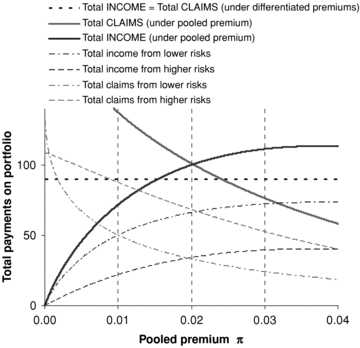
Scenario 2: Higher Loss Coverage Under Pooled Premium: (λ1, λ2) = (0.5, 1.1)
Figure 1 can be interpreted as follows. The horizontal line is a reference level representing total premiums (and, by assumption, total claims) when accurate risk-differentiated premiums are charged to the two populations. All other curves represent premiums or claims when a single rate of premium π is charged to both populations. On the left-hand side of the graph, where the single rate of premium π is low, demand for insurance at this price is high, and so total claims paid are high. Because of the low premium, total premiums collected are low; the market is far from equilibrium and insurers make large losses. Insurers will therefore increase the pooled premium, and some customers will leave the market. As customers leave the market, total claims decrease monotonically (the downward sloping curve), but total premiums collected increase because the increase in the premium rate outweighs the number of customers leaving the market. So the curve of total premium income slopes upward, at least initially.
The intersection of the darker curves for total premiums and total claims represents a pooling equilibrium. This equilibrium is at a higher level of total premiums and total claims than in the risk-differentiated market; that is, loss coverage has been increased.
The two pairs of lighter curves show total premiums and total claims for populations 1 (low risk) and 2 (high risk) separately. The heavier curve for total premiums can then be seen as the sum of the two lighter curves for total premiums in each of the two populations and similarly for the claims curves. The lighter total claims and total premiums curves intersect at π= 0.01 (for population 1) and at π= 0.04 (for population 2); this is as expected.
To implement Scenario 3 from the “Examples” section, the only change we need to make is to increase the price elasticity parameter λ1 in the lower risk group. Figure 2 illustrates that (λ1, λ2) = (0.8, 1.1) approximately reproduces Scenario 3 (an 11 percent deterioration in loss coverage under restricted risk classification). The more elastic demand in the lower risk population leads to lower loss coverage (a worse result) under restricted risk classification.
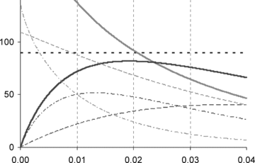
Scenario 3: Lower Loss Coverage Under Pooled Premium: (λ1, λ2) = (0.8, 1.1)
Interpreting the Elasticities


Using the above formulas we can calculate the actual elasticities of demand in higher and lower risk populations at the equilibrium pooled premium. These are 0.63 and 0.40 for the higher and lower risk populations, respectively, in Figure 1 and 1.59 and 0.62, respectively, in Figure 2. These values deviate in the expected directions from the fair-premium elasticities: higher for the lower risk population (for whom the equilibrium pooled premium is dear) and lower for the higher risk population (for whom the equilibrium pooled premium is cheap).
An Extreme Equilibrium
Figure 3 illustrates the result for very elastic demand (λ1, λ2) = (1.4, 1.1). The total premiums and total claims curves intersect very close to the terminal value for π, with virtually all the lower risks out of the market. Note that while this is technically possible, the high elasticity in the lower risk population which is required to generate this result may be unlikely.
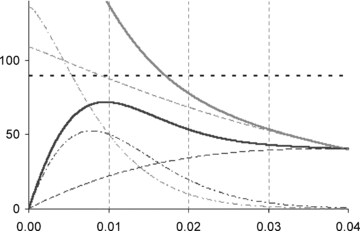
An Extreme Equilibrium: (λ1, λ2) = (1.4, 1.1)
Sensitivity of Loss Coverage to λ1 and λ2
In 1-3, a constant λ2= 1.1 was used as a convenient value to approximately reproduce the scenarios given in the “Examples” section. Loss coverage fell when λ1 was increased (i.e., the lower risk population was made more sensitive to price), that is, writing L for loss coverage, ∂L/∂λ1 < 0. This is a general result. If we start in a pooling equilibrium and elasticity in the lower risk group increases slightly, demand from them at the previous equilibrium price decreases, implying a slightly higher pooled premium; this in turn implies that demand from higher risks must also drop slightly, and so loss coverage at the new equilibrium is unambiguously lower. For λ1 around the values used in our examples, loss coverage rises when λ2 is increased (i.e., the high risk population is made more sensitive to price), that is, ∂L/∂λ2 > 0. However, although this applies in all our examples so far, it is not a universal result. If we start in a pooling equilibrium and the elasticity in the higher risk group increases slightly, demand from them at the pooled price increases, implying a slightly higher premium; this in turn implies that demand from lower risks must decrease slightly. The effect on loss coverage could be an increase or decrease, depending on whether the increased demand from higher risks at the new equilibrium outweighs (in loss coverage terms) the reduced demand from lower risks. ∂L/∂λ2 > 0 is the usual result when using plausible elasticity parameters, but for high values of λ1 the sign can be reversed; an example is given later in the article.
In our examples, results are much more sensitive to changes in λ1 than to changes in λ2. This effect is illustrated in Figure 4, which shows loss coverage under restricted risk classification as a function of λ2 for four values of λ1 between 0.4 and 0.7. The horizontal line in each graph represents loss coverage under accurate risk classification. As λ1 increases from graphs 1 to 4, the line representing loss coverage under restricted risk classification as a function of λ2 moves downward and reduces in slope. For λ1= 0.4, an improvement in loss coverage under restricted risk classification requires only λ2 > 0.33. For λ1= 0.7, an improvement in loss coverage requires λ2 > 1.25. The greater sensitivity to λ1 depends on the relative numbers and risks in the two populations, but it is a typical result for the “normal” scenario of a larger population with a lower risk.

Loss Coverage as a Function of λ2 for Four Values of λ1
Sensitivity of Equilibrium Premia to λ1 and λ2
Figure 5 shows the equilibrium premia π* corresponding to each of the panels in Figure 4. As λ1 increases from graphs 1 to 4, the line representing the pooled premium under restricted risk classification as a function of λ2 moves upward and increases in slope. The horizontal line at 0.015 in each graph represents the population-weighted average premium. The distance between the slope and the horizontal line represents a conventional concept and measure of the severity of adverse selection: the extent to which the equilibrium pooled premium exceeds the population-weighted average premium. But the policymaker in this article is concerned with loss coverage; comparing the panels in Figure 4, we see that adverse selection as illustrated in Figure 5 can sometimes be associated with higher loss coverage than under risk-differentiated premiums.
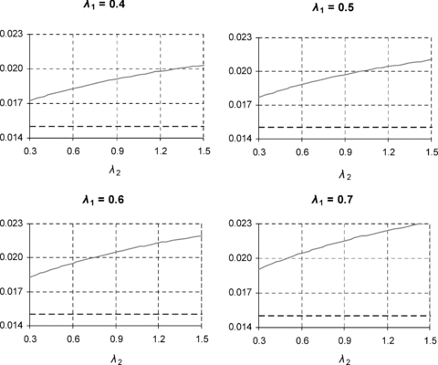
Equilibrium Premium Under Restricted Risk Classification as a Function of λ2 for Four Values of λ1
It is also of interest to note that in Figure 5, the equilibrium premium is increased by any increase in demand elasticity, in either risk group. For the higher risk group, this is represented by the upward slope of premium line; for the lower risk group, it is represented by the upward movement of the premium line across the progression of the four graphs. Thus, under the conventional paradigm where all adverse selection is viewed as negative, any increase in demand elasticity, in either risk group, would be viewed as negative. But in Figure 4, while increases in demand elasticity in the lower risk group reduce loss coverage, increases in demand elasticity in the higher risk group increase loss coverage. Thus, for a policymaker with a loss coverage objective, an increase in demand elasticity in the higher risk group may not be negative.
An Unstable Equilibrium
We noted above that ∂L/∂λ1 < 0 and that this appeared to be a general result, but while ∂L/∂λ2 > 0 in all our examples, we could not say that this was a general result. It is of some technical interest to show a counterexample where ∂L/∂λ2 < 0. This does not appear to arise for relative population sizes and fair-premium take-ups assumed earlier in the article. However, if we assume a smaller higher risk population, or assume that fair-premium take-up in the higher risk population is lower—that is, we set a lower value for τ2—then we can obtain the required counterexample. For example, Figure 6 and Figure 7 show results for τ2= 0.25 and (λ1, λ2) = (1.1, 1.2). This is a rather unstable equilibrium, where small changes in λ1 can lead to relatively large changes in the equilibrium premium. Graphically, in Figure 6, small movements in the total income and total claims curves can substantially change the π-value at their intersection, and correspondingly, in Figure 7, the slope of the equilibrium premium line as a function of λ2 is steep.
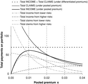
Equilibrium With τ2= 0.25 and (λ1, λ2) = (1.1, 1.2)
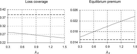
Loss Coverage and Equilibrium Premium as a Function of λ2 for λ1= 1.1
It is also technically possible to specify models of the type used in this article so that curves broadly similar to those in Figure 6 intersect more than once along their downward slope, illustrating the nonuniqueness of the solution to the zero-profits condition. However, for many relative population sizes and relative risks, multiple solutions cannot be generated, and where they can, it generally requires rather implausible parameter values for (λ1, λ2).5
An Application to the UK Life Insurance Market
This section of the article speculates about the possible consequences for loss coverage of a change in the UK life insurance market from the present rating approach to a less differentiated approach. In underwriting life insurance, UK life insurers typically divide applications into three broad categories. Most applicants are offered the insurer's “standard” rate for their age, sex, and smoking status; a smaller group is offered a range of higher rates to reflect medical conditions, occupational hazards, etc.; and a few applicants are declined.6 A recent survey (Bennett, 2006) that received responses from about 80 percent of UK life offices currently accepting new business suggests that currently around 90 percent of applicants for life insurance are offered standard rates, around 8 percent are offered higher rates, and around 2 percent of applications are declined. I consider combining the first two groups, with the last group continuing to be declined under the new approach; all figures for loss coverage and size of market from here onward are calculated disregarding the 2 percent excluded under both regimes.
I have no data on the distribution by amount of rating within the rated lives, but reinsurance manuals and a standard underwriting textbook (Brackenridge, 1998) recommend additional mortality for various conditions ranging from 50 percent (occasionally 25 percent) to 400 percent above standard mortality; the ratings for more common conditions tend to be toward the lower end of this range. In the absence of better information, I assume that the rated class as a whole can be modeled by a force of mortality 100 percent above standard. For term insurance, the additional premiums will be broadly proportional to the rating. This suggests the parameters P1= 90, P2= 8, and μ1= 0.001, μ2= 0.002.
Under the present risk-differentiated approach around 50 percent of the population are reported to pay some life insurance premiums (Association of British Insurers, 2007); this suggests 0.9τ1+ 0.08τ2= 0.5. I have no data for τ2. I think it would probably be somewhat lower than τ1 because lives that are (or expect to be) quoted higher ratings are probably discouraged from obtaining insurance, and the risk-differentiated premium can appear unreasonably high relative to other expenditures. I have set τ2= 0.4 and hence τ1= 0.52. (The results are not very different for, e.g., τ2= 0.5.) I assume that the 90:8:2 proportions of decisions on applications actually seen under risk rating are representative of the underlying population of potential applicants under community rating.
The graphs in Figure 8 show loss coverage with restricted risk classification as a function of λ2 for four values of λ1 between 0.4 and 0.7. The horizontal line in each graph represents loss coverage under accurate risk classification. The pattern of results is similar to those in Figure 4, although the change in the position and slope of the line as one moves from one graph to the next is smaller.
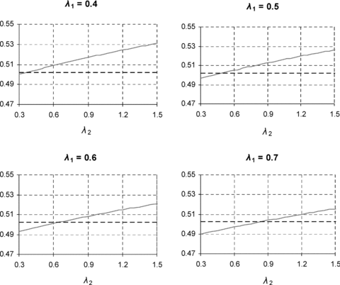
Loss Coverage as a Function of λ2 for Four Values of λ1
In this model, with plausible parameter values, when higher loss coverage is achieved it is usually with a lower total number of policies sold than under accurate risk classification. Higher loss coverage corresponds to a larger market in terms of premium income, but a smaller market in terms of numbers of polices. This reflects the shift of coverage away from lower risks and toward higher risks: “more policies are sold to the right people,” that is, people more likely to suffer loss. For (λ1, λ2) = (0.4, 0.65), which gives an improvement in loss coverage of 1.6 percent, the reduction in number of policies issued is 0.7 percent. For (λ1, λ2) = (0.7, 1.2), which also gives an improvement in loss coverage of 1.6 percent, the reduction in number of policies issued is 2.5 percent. The latter pair of elasticity parameters implies a more marked shift of coverage toward higher risks when risk classification is restricted, and hence the same increase in loss coverage corresponds to a larger fall in number of policies issued. For low λ1 a sufficiently high λ2 can lead to an increase in loss coverage with a small increase in policies sold when risk classification is restricted. For λ1= 0.4, any λ2 > 0.95 leads to both an increase in loss coverage and an increase in number of policies sold. For example, the parameters (λ1, λ2) = (0.4, 1.1) give a 4.0 percent increase in loss coverage and a 0.3 percent increase in number of policies sold. But this pattern is less typical; more often, an increase in loss coverage is associated with a reduction in number of policies sold.
It is sometimes observed that even in markets where risk classification is unregulated, insurers in practice seem to disregard some information that is observable at minimal cost and apparently relevant to the risk. For example, health insurance and long-term care insurance often seem to be based on broad bands that ignore relevant information such as gender; retail creditor insurance is often operated with very little classification of risk; and the large majority group of customers traditionally offered standard rates in the UK life insurance market probably includes a good deal of observable heterogeneity. Commonly suggested explanations of this include cultural factors and tradition, or lack of pricing sophistication. Another possible explanation suggested by this article is that insurers collectively may prefer to maximize premium income rather than number of policies sold. A relatively undifferentiated premium schedule may better achieve this objective than accurate risk pricing.
In practice, it is very unlikely that public policy would mandate that life insurance risk classification is reduced to an accept/reject decision (and if it did, the proportion of lives rejected by insurers might increase rather than staying the same as in this model). However, the model in this section illustrates two key ideas:
- •
the relevance of demand elasticities in determining the outcome of changes in risk classification;
- •
the distinction between market size as measured by number of policies issued, which in this model (with plausible parameter values) usually falls when risk classification is restricted, and loss coverage, which may rise or fall when risk classification is restricted. Loss coverage rises if the shift in coverage toward higher risk lives following a restriction in risk classification outweighs any fall in number of policies issued.
The model also provides a mental framework for thinking about more limited restrictions on risk classification. A small reduction in gradation in risk classification may induce a modest increase in adverse selection and an increase in loss coverage. A more drastic reduction in gradation in risk classification may induce higher levels of adverse selection and a reduction in loss coverage. Alternatively, if we are starting from a different point, some increase in the gradation of risk may be required to increase loss coverage. From the public policymaker's perspective, I suggest it may be a question of degree: how to induce the level of adverse selection that maximizes loss coverage.
Conclusions and Further Research
This article has suggested that from a public policy perspective, adverse selection may not always be adverse. A public policymaker concerned with risk classification in markets where insurance is seen as having social benefits may wish to consider the criterion of loss coverage. In the models in this article, restrictions in risk classification usually lead to a reduction in number of policies sold but can lead to either an increase or decrease in loss coverage. A public policymaker may wish to impose some restrictions on risk classification and induce some degree of regulatory adverse selection and possibly a smaller total number of policies sold, if this leads to an increase in loss coverage.
Whether restrictions on risk classification lead to an increase or decrease in loss coverage depends on the relative sizes of higher and lower risk populations, their relative risks, and price elasticities of demand for insurance from each population. For given relative population sizes and relative risks, restrictions on risk classification lead to an increase in loss coverage if the price elasticity of demand in the lower risk group is sufficiently low, compared to that of the higher risk group.
There seems to be little information on price elasticities of demand for insurance, and certainly none that I know of on any differential elasticities for higher and lower risk groups. Although there are some reasons for thinking that price elasticity of fair-premium demand would indeed generally be lower in lower risk groups, any empirical investigations of this point would be of considerable interest.


