Risk-Management and Risk-Analysis-Based Decision Tools for Attacks on Electric Power
Abstract
Incident data about disruptions to the electric power grid provide useful information that can be used as inputs into risk management policies in the energy sector for disruptions from a variety of origins, including terrorist attacks. This article uses data from the Disturbance Analysis Working Group (DAWG) database, which is maintained by the North American Electric Reliability Council (NERC), to look at incidents over time in the United States and Canada for the period 1990–2004. Negative binomial regression, logistic regression, and weighted least squares regression are used to gain a better understanding of how these disturbances varied over time and by season during this period, and to analyze how characteristics such as number of customers lost and outage duration are related to different characteristics of the outages. The results of the models can be used as inputs to construct various scenarios to estimate potential outcomes of electric power outages, encompassing the risks, consequences, and costs of such outages.
1. INTRODUCTION
Disruptions to the power grid are an ongoing concern for risk management in the energy sector. Although there have, to date, not been any terrorist attacks on the power grid in the United States or Canada by a foreign entity, such attacks are common in other countries. The consequences of these disruptions include effects on the economic and health status of the country. It is thus important to try to understand the characteristics of disruption to the power grid, so that reasonable assessments of the risks associated with such disruptions can be quantified.
In this article, various forms of statistical regression analyses are used to model the characteristics of power outages in the United States and Canada. None of these disruptions are a result of terrorist activity, but understanding the effects of “typical” disruptions would make it possible to estimate the effects of a terrorist-based disruption, especially since there is enough of a similarity between the types of components disrupted in both types of events (as described below). The potentially large effects of such disruptions, as evidenced by the roughly 50 million people affected by the August 14, 2003 outage lasting an average of two days in most places in the northeastern United States and southeastern Canada, and the roughly 100,000 people affected by the one-week July 18, 2006 outage in Queens neighborhoods in New York City (Newsday, 2006), reinforces the importance of understanding the potential implications of terror-related outages. The resultant regression models allow us to see what characteristics of an event are associated with its duration and how many customers are affected. On the basis of these models, predictions (and probability intervals for those predictions) can be made for different disruption scenarios that allow for quantitative assessments of potential risks and consequences of attacks on the power grid regardless of the source of the attack. Of course, these predictions are also useful in the context of nonterrorist disruption of the power grid, such as from the severe weather effects of tornadoes, hurricanes, and winter storms.
1.1. Analogies Between Terrorist and Nonterrorist Disruptions of Electric Power Systems
An analysis of selected data from the National Memorial Institute for the Prevention of Terrorism (MIPT) database (http://www.mipt.org) indicates that in a 10-year period between 1994 and 2004, there were more than 300 terrorist attacks around the world against electricity infrastructure alone (Zimmerman et al., 2005). The analogy between international terrorist attacks and domestic nonterrorist disruptions of electric power systems is supported by a comparison of the MIPT database of international attacks and the Disturbance Analysis Working Group (DAWG) database, maintained by the North American Electric Reliability Council (NERC) for North American disruptions. This comparison indicates similarities between components disrupted by terrorist attacks outside of North America and nonterrorist disruptions within North America. The most common components disrupted in both cases were transmission lines and towers, accounting for about 90% of North American disruptions and about two-thirds of international terrorist-related disruptions (Zimmerman et al., 2005, Table 1, p. 19). These similarities, at least at the component or consequence level between terrorist and nonterrorist electricity disruptions, support using nonterrorist databases to estimate the potential consequences of terrorist attacks on electricity.
| Cause | Code | United States | Canada | ||
|---|---|---|---|---|---|
| Frequency | Percent | Frequency | Percent | ||
| Capacity shortage | C | 15 | 3.8 | 1 | 1.0 |
| Crime | Crime | 9 | 2.3 | 5 | 5.2 |
| Demand reduction | D | 5 | 1.3 | 0 | 0.0 |
| Equipment failure | E | 111 | 28.0 | 39 | 40.2 |
| Fire | F | 12 | 3.0 | 0 | 0.0 |
| Human error | H | 21 | 5.3 | 15 | 15.5 |
| Operational error | O | 5 | 1.3 | 1 | 1.0 |
| Natural disaster | N | 6 | 1.5 | 0 | 0.0 |
| System protection | S | 6 | 1.5 | 2 | 2.1 |
| Third party | T | 6 | 1.5 | 1 | 1.0 |
| Unknown | U | 10 | 2.5 | 2 | 2.1 |
| Weather | W | 190 | 48.0 | 31 | 32.0 |
| Total | 396 | 100.0 | 97 | 100.0 | |
That research further explored grid configurations (particularly at the transmission level) that could contribute to vulnerability and the degree of the consequences of a disruption for major cities. In short, certain cities are more vulnerable than others by virtue of their reliance on transmission lines that enter the city from just one or two directions (Zimmerman et al., 2005, pp. 15–17). This point informs the choice of application areas later in this article.
1.2. Literature Review of Event-Based Analyses Modeling of Electric Power Outages
The major contribution of this work is to provide a statistical regression-based approach using trend data to model the consequences and severity of outages from the characteristics of outage events. This will serve as a basis for decision tools that enable users to estimate the probability of certain impacts of outages occurring, and tailor these estimates to specific geographic areas. To our knowledge, this type of approach using statistical regression models has not been applied to estimating these dimensions of electric power outages.
As summarized by Zimmerman et al. (2005), one body of literature contains extensive analyses of electric power outage event data (see, for example, Amin, 2004; Carreras et al., 2002; Chen et al., 2001; Liao et al., 2004), but does not use statistical regression analysis. Another body of literature has attempted to model outages, but primarily by building scenarios and/or through grid network disruption estimates (see, for example, Ezell et al., 2000a, 2000b; Haimes, 1981; Salmeron et al., 2004; Lemon & Apostolakis, 2004; Apostolakis & Lemon, 2005). A third related literature uses scenario-based or simulation-based modeling of infrastructure interdependencies in general (see, for example, Garrick et al., 2004; Martz & Johnson, 1987; Masiello et al., 2004; Paté-Cornell & Guikema, 2002).
Several studies have analyzed data from the DAWG database using methods that are different from those used in this article and for a different purpose. Chen et al. (2001) analyzed the data for the period 1984–1999 and constructed blackout time series signals. The size of the blackouts is represented by the amount of power lost in megawatts, the number of customers affected, and the duration of the outage or restoration time. The time series include data for every day of the period with zero every day except for the days when blackouts occurred. The time series is then used to explore whether the data have a power law distribution by using a cumulative distribution function (CDF). In addition, the scaled windowed variance (SWV) method is used to estimate the Hurst or scaling exponents of the various time series and its suitability to the data is discussed.
Carreras et al. (2002) also analyzed DAWG data for the period 1984–1998 to examine whether the complex dynamic of the blackouts is governed by self-organized criticality (SOC). The authors constructed times series with the resolution of a day for the number of blackouts and for three measures of blackout size: energy unserved, amount of power lost in megawatts, and number of customers affected. The data are used to explore dependencies in the time domain. They also find a power law tail of the probability distribution functions (PDF). The authors use the rescaled range statistics (R/S statistics) to calculate Hurst exponents for the different measures of blackout size. Similarly, Talukdar et al. (2003) also use DAWG data for the period 1984–2000 to show that large blackouts, such as those exceeding 500 megawatts lost, can be described by a power law whereas the smaller blackouts follow an exponential curve. These types of analyses of the DAWG data are very different in purpose and methods to the analyses presented in this article and described in the following sections.
2. DATA
The analyses presented in this article use data from the Disturbance Analysis Working Group (DAWG) database, which is maintained by the North American Electric Reliability Council (NERC). The database has commonly been used by researchers to analyze power outages and various attributes of the grid, while recognizing some of the shortcomings of the database (Apt, 2005; Talukdar et al., 2003; Chen et al., 2001; Carreras et al., 2002; Amin, 2004). Data are collected on a voluntary basis, implying the possibility of unknown biases in the outages reported, as well as potential changes in the way the data have been reported over time. The U.S. Department of Energy (2003) also has a database of outages, but for the sake of temporal consistency and the ability to tap a database spanning a longer time period, the DAWG database was used throughout.
The data used in this article are for disturbances to the electric power grids in the United States and Canada for the period 1990–2004 (in this article the terms disturbances, incidents, events, and outages are used interchangeably). Information from the entries in the DAWG database was used to create a data set with a number of variables that characterized each event. These included outage duration measured in hours, number of customers lost, and megawatts lost. All three of these variables are extremely long right-tailed.
The mean duration of an outage in the United States was more than 40 hours, while the median duration was 8 hours; corresponding numbers for Canada are noticeably smaller, being 7.3 and 0.8 hours, respectively (but still long right-tailed). Similarly, mean and median customer losses were 175,346 (mean) and 67,765 (median) for the United States and 58,897 (mean) and 1 (median) for Canada, respectively, and mean and median power loss (in MW) were 786 (mean) and 250 (median) for the United States and 513 (mean) and 258 (median) for Canada, respectively. For this reason, all these variables are analyzed in the log scale.
The cause of the incident is also a potentially important predictor of the magnitude and characteristics of an outage and also the construction of analogies between nonterrorist and terrorist consequences. In addition, the relative importance of these causes can change over time and that could have important implications for policies aimed at minimizing the risk of power outages and for the construction of scenarios that explore economic costs associated with outages. Table I gives the distribution of the different causes for the incidents.
A proxy for population density in the area of the outage was also included in the data for the purpose of regression modeling. This was approximated by using population density for the state where the outage occurred in the United States and for the province where the outage occurred in Canada. It should certainly be noted that since most outages cover geographic regions smaller than a state or province and within a given state population density can be highly variable, this is only a crude proxy for the local population density.
An additional measure added to the data was the number of customers served by the utility or utilities affected by each outage. This information was compiled from the U.S. Department of Energy, Energy Information Administration's Annual Electric Power Industry Report (U.S. Department of Energy, 2003), individual utility pages on the Internet, and electric power trade associations.
3. METHODS
The first set of analyses included in this article refers to models of counts of incidents over time. The standard model for count response data is the Poisson regression model, but this model imposes the restriction that the mean response and the variance of the response be equal. For the data examined here, there is clear overdispersion, with the variance larger than the mean. This is a common occurrence when there is unmodeled heterogeneity in the data (that is, the time periods are different from each other in ways that are unknown to the analyst). For this reason, the analyses here are based on negative binomial regression, which accounts for this overdispersion. See Simonoff (2003, ch. 5), for further discussion of these points. The data for number of incidents were aggregated into three- and six-month periods, approximating seasons, to examine whether there are time trends.
The second set of analyses refers to event-level data. These event analyses account for characteristics unique to the particular event, such as its cause and location, through regression modeling. Two different kinds of models were used for the event-level analyses. In the case of number of customers lost, there are two kinds of events: those resulting in zero customers lost, and those with nonzero customers lost. It is important to distinguish these two types of events since they have different characteristics. Hence, the data were modeled in two parts. First, the characteristics related to whether an incident has zero or nonzero customers lost are examined. Then, given that the number of customers lost is not zero, the characteristics that help predict the actual number of customers lost are determined.
The first part of the analysis is based on logistic regression. In a logistic regression, the response variable is binary (in this case, whether or not the event had zero customer loss), and a binomial distribution is used to represent its random character. The probability of an event having zero customer loss, p, is related to predictors through the odds, p/(1 −p); specifically, the logarithm of the odds is modeled as a linear function of the predictors (Simonoff, 2003, ch. 9).
For the second part of the analysis, weighted least squares (WLS) was used to correct for nonconstant variance in the data. In the WLS analysis, the events from causes with less variability, such as capacity shortage and fire, are weighted higher, while those from causes with more variability, such as equipment failure and system protection, are weighted lower. Weighted least squares regression was also used to model logged duration of an outage.
Further details on the U.S. portion of this analysis can be found in Simonoff et al. (2005).
4. RESULTS
4.1. Incidents Over Time
The first part of this analysis consists of looking at the number of incidents aggregated over six-month periods for 1990–2004. The negative binomial model fits the data well. For the U.S. data the deviance equals 15.3 on 12 degrees of freedom ( p= 0.23, not rejecting the fit of the model). The estimated annual increase in incidents implies a 7.2% annual increase in incidents. For Canada, the model also fits the data reasonably well (the deviance is 32.3 on 24 degrees of freedom, p= 0.12), and it implies an estimated 8.2% annual increase in incidents.
Examining the data at a seasonal (three-month period) level allows for the inclusion of different levels for different seasons. In these analyses, winter is defined as December through February, spring as March through May, summer as June through August, and autumn as September through November. The results for the seasonal analysis are summarized in Fig. 1 for the United States and in Fig. 2 for Canada. The winter points (labeled “w”) and line (dotted line) are in blue, the spring points (labeled “p”) and line (dashed line) are in green, the summer points (labeled “u”) and line (solid line) are in red, and the autumn points (labeled “a”) and line (dotted-and-dashed line) are in orange.
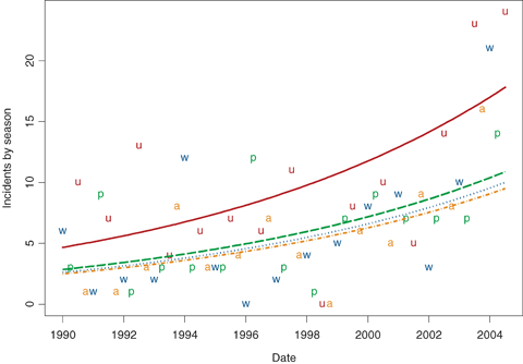
Plot of number of incidents in United States versus time by season, with estimated expected counts by season superimposed on the plot.
Key: The winter points (w) and dashed line are in blue, the spring points (p) and dotted line are in green, thesummer points (u) and solid line are in red, and the autumn points (a) and short dashed line are in or-ange. Calculations by the authors.
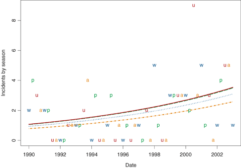
Plot of number of incidents in Canada versus time by season, with estimated expected counts by season superimposed on the plot.
Key: The winter points (w) and dashed line are in blue, the spring points (p) and dotted line are in green, thesummer points (u) and solid line are in red, and the autumn points (a) and short dashed line are in orange.
The negative binomial models fit the data adequately. For the U.S. model, the deviance is 66.5 on 53 degrees of freedom ( p= 0.10) and implies an estimated 9.7% annual increase in incidents given season, which is highly statistically significant ( p < 0.0001). For Canada, the model fits the data barely adequately (the deviance is 60.4 on 46 degrees of freedom, p= 0.08). The model implies an estimated 9.6% annual increase in incidents given season, virtually the same as for the U.S. data.
There are several plausible explanations for the observed annual increase in incidents. Electricity demand has increased steadily over time (North American Energy Working Group, 2006), and this increased demand puts more strain on the electricity grid. In addition, Lerner (2003) gave several reasons why the deregulation of the electricity markets in the United States and Canada starting in the 1990s would be (and was) expected to lead to more blackouts. Specifically, while long-distance energy transfers were rare before deregulation, and were used mainly in emergencies, they have now become commonplace. Such transfers are much more physically complex, involve more complex interconnections between the large physical subsections of the power grid, and introduce capacity limits, resulting in greater chances of unanticipated changes in loads on generators and transmission lines, and hence blackouts. These problems were compounded by energy traders who deliberately blocked competitors' access to the power grid, artificially driving up prices while also increasing stress on the system. Utility companies have also cut staff, resulting in overextended workers and reduction in basic maintenance. Finally, as a result of many of these factors, the grid has become far more interconnected, so that a failure in one part of a system is likely to affect others. Moreover, many more activities are now interconnected with electric power as well, and these interdependencies have the potential for increasing the consequences of an electric power failure (Zimmerman & Restrepo, 2006; Zimmerman, 2006).
While the winter, spring, and autumn estimated rates for the United States are similar to each other (with autumn having a rate that is slightly lower), summer has a noticeably higher rate of incidents. The similarity in rates across seasons is presumably from different weather effects operating in each season: snow and ice in the winter, thunderstorms in parts of the United States in spring, and, most importantly, thunderstorms and intense heat (with corresponding air conditioner use) in the summer (and the lack of all of these factors in the autumn; we might have expected evidence of a hurricane effect in autumn, but only Hurricane Floyd in 1999 and Hurricane Isabel in 2003 show up as noteworthy). The difference between the summer rate and that of the other seasons is highly statistically significant, but, more importantly, corresponds to an important effect in practical terms, since the estimated number of incidents is 60–80% higher in summer than in the other seasons, given the year. In the case of Canada there is little evidence of a season effect (presumably because of the less extreme summer temperatures in Canada), although summer does again have the highest estimated incident rate.
In addition to looking at the total number of incidents over time, similar analyses were made for those incidents with nonzero customer loss and nonzero megawatts lost. Such incidents are of particular importance, since these are the ones that actually affect customers. Overdispersion is evident in all of the models, so all analyses are based on the negative binomial model. For the U.S. data the estimated annual increase in incidents with nonzero MW loss is 10.0%, which is highly statistically significant ( p < 0.0001), with an estimated 65–130% higher rate for summer than for the other seasons. The summer effect is stronger than it was in the model for number of incidents. While more than 90% of the summer incidents had nonzero MW loss, roughly one upon four of the incidents in the autumn had zero MW loss. That is, nonzero MW incidents are more likely in the summer, thereby strengthening the “summer effect.”
The results for the Canada model in terms of incidents with nonzero MW loss are in direct contrast to the situation using all of the incidents, and also in contrast to the results for the U.S. data. There is no evidence of a time trend in the nonzero MW Canadian incidents. The implication of this is that the rate of zero MW loss incidents in Canada has been increasing in recent years. From 1990 to 1994, the proportion of Canadian incidents with zero MW loss was never more than 25% (among those for which MW loss was recorded), while from 1995 to 2002, in five of the eight years at least 30% of the incidents had zero MW loss. It should be noted, however, that the estimated increase in incident rate of 3.5%, while smaller than that in the United States (6.0%), is not significantly different from that value. When season is introduced, the model implies an estimated 1.7% annual increase in incident rate given season, which is not statistically significant, and an estimated 75% higher rate for summer than for the other seasons, although the summer effect is also not statistically significant.
The model for incidents with nonzero customers lost in the United States implies an estimated 14.0% annual increase in incident rate ( p < 0.000001), and an estimated 75–135% higher rate for summer than for the other seasons. The summer effect is similar to that for the nonzero MW loss data, but the pattern is a little more complicated: both summer and winter have lower rates of incidents with zero customer loss compared to spring and autumn, so the estimated relative chances of incidents in those seasons compared to spring and autumn are now higher. Overall, while removing the zero MW loss incidents has relatively little effect on the estimated annual increase in incident rate, removing the zero customer loss incidents has a stronger effect on the estimated annual increase of rates, increasing it to 12–14%.
The results of the model for Canada are different from those of the United States, since there is little evidence of any relationship with either season or time for incidents with nonzero customers lost. When focusing on incidents with nonzero customer loss, the rate of incidents in Canada is, if anything, decreasing over time, while that in the United States is increasing. This is in contrast to the situation when looking at all incidents, where the rate is going up at a similar rate in both countries. As was noted earlier, the reason for this is the difference in the two countries in the likelihood of an outage having zero customer loss.
The generally less-serious outcomes of Canadian incidents compared to incidents in the United States (such as shorter typical duration, no increase over time in incidents that resulted in nonzero customer loss or nonzero power loss) warrants further comment. Although the electricity grids in the United States and Canada are strongly interconnected, there are differences between the two countries that could account for this pattern. The great majority (almost 85%) of the incidents in Canada were in provinces that are net exporters of electricity (North American Energy Working Group, 2006). Incidents in such provinces occur in areas of excess supply of electricity, which can be more easily used to recover from or compensate for local outages. The proportion of incidents in provinces that are net exporters of electricity was higher in recent years than in earlier ones (North American Energy Working Group, 2006), which could be a factor in why the number of more serious incidents (nonzero MW loss and/or customer loss) are if anything slightly decreasing in Canada, rather than increasing (as they are in the United States).
The distribution of types of power plants is very different in the United States and Canada. While roughly half of electricity generation in the United States comes from coal-fired plants, more than half of electricity generation in Canada comes from hydropower (estimated 2005 values) (North American Energy Working Group, 2006). Hydroelectric plants have an abundant and readily available local fuel supply with the exception of rare periods of drought, while that for coal-fired plants is limited and difficult to move. This clearly has an effect on recovery time from an outage. As noted by Lerner (2003), hydroelectric power plants in Ontario and Quebec were regularly involved in long-distance power transfers before the advent of deregulation, so it is reasonable to speculate that they have been better able to handle the stresses that come from such transfers noted in Section 4.1 than other types of plants.
Another explanation for the relatively good performance of the power grid in Canada is an economic one. Electricity demand is growing more slowly in Canada than in the United States, even though the economies of the two countries are growing at a similar rate (North American Energy Working Group, 2006). As noted earlier, increased demand would be expected to lead to increased stress on the system, and less demand growth would be expected to correspond to better results.
4.2. Event-Level Analyses
In this section, we present the results of weighted least squares regression models that use characteristics of each event, such as cause, season, and a proxy for population density, to gain a better understanding of the factors that affect the number of customers lost and duration of an outage.
4.2.1. Number of Customers Lost During an Outage
The first analysis refers to number of customers lost, and the first issue explored is whether an incident has zero or nonzero customers lost and the factors that affect this outcome. As mentioned earlier, these analyses used logistic regression. The U.S. data suggest that there is little difference in the distribution of logged total customers served by a utility for incidents with nonzero customer loss versus for incidents with zero customer loss. As might be expected of apparently more serious incidents, longer incidents are associated with nonzero customer loss. Also, incidents in more densely populated states are more likely to have nonzero customer loss. In addition, there is a strong pattern where incidents earlier in time are more likely to have zero customer loss.
The other potential predictors for the number of customers lost during an outage are season and cause of the outage. In the United States, zero loss incidents are more common in the spring (26.3%) and autumn (21.3%), and less common in the summer (15.3%) and winter (13.9%). These are not, however, very strong effects. Weather-related incidents are very likely to have nonzero customer loss, no doubt at least in part because of the disruption of overhead transmission and distribution lines by fallen trees (which can occur in either summer or winter storms), and are not fixed quickly or at least before customers are affected. Capacity shortage, system protection, and unknown causes are also strongly associated with nonzero customer loss, but this is based on far fewer incidents. Equipment failure is noticeably less related to nonzero customer loss (while also having a large number of incidents). More atypical causes that are less associated with nonzero customer loss include fire, human error, natural disaster, and operational error; crime, demand reduction, and third-party cause have zero customer loss rates more than 50% (although again, based on few incidents).
For the U.S. model, logged duration, logged population density, a time trend (days since 1990), and cause are significant predictors of whether an event is associated with zero or nonzero customer loss, but season is not. The coefficients produced by the model have the following interpretations. A 1% increase in the duration of an incident is associated with an estimated 0.3% decrease in the odds that an incident will have zero customer loss, holding all else in the model fixed. A 1% increase in the state population density is associated with an estimated 0.6% decrease in the odds that an incident will have zero customer loss, holding all else in the model fixed. The estimated annual decrease in the odds of an event having zero customer loss is 11.3%, holding all else in the model fixed. Finally, given the other predictors, crime, demand reduction, and third-party cause are strongly associated with zero customer loss, while operational error, system protection, and weather are strongly associated with nonzero loss.
The analysis of the Canada data is based on fewer observations. Unfortunately, for 17 of the incidents, a customer loss value was not available (and hence it can't be known if the customer loss was zero or not). In addition, for 26 other incidents, (logged) duration was not available. Together, this means that the Canada model is based on only 55 data points.
For these data, logged total customers served by the utility has an inverse relationship with the probability that an outage has zero customer loss; a 1% increase in the customer base is associated with a 1.1% decrease in the odds that an incident has a zero customer loss. In contrast, in the United States logged total customers served by the utility did not appear in the corresponding (simplified) logistic regression model. As was true in the United States, longer outages are associated with smaller likelihood of zero customer loss; a 1% increase in duration is associated with a 0.5% decrease in the odds that an outage has zero customer loss. In contrast to the United States, outages in denser areas of Canada (provinces rather than states here) are associated with a higher chance of it being a zero customer loss incident, as a 1% increase in population density is associated with a 1.4% increase in the odds of having zero customer loss, holding all else fixed (the relationship was in the opposite direction in the U.S. data). As was noted earlier, in direct contrast to the situation in the United States, zero customer loss incidents are becoming more common in Canada, corresponding to an estimated 31.5% annual increase in the odds that an outage has zero customer loss, given the other predictors. Winter and especially summer incidents are less likely to have zero customer loss, although this does not appear to be statistically significant. Compared to the “other” category, given the other predictors, crime and weather are more likely to occur with zero customer loss incidents, while equipment failure and human error are less likely. These are not very similar to the patterns in the U.S. data.
Table II summarizes the differences between the two countries with respect to the model in terms of the relationship with the probability that an incident has zero customer loss.
| Effect | United States | Canada |
|---|---|---|
| Logged total customers | No relationship | Inverse relationship |
| Logged population density | Inverse relationship | Direct relationship |
| Time (days since 1990) | Inverse relationship | Direct relationship |
| Primary cause | Weather lower probability than equipment failure | Weather higher probability than equipment failure |
The second aspect of customer loss explored is the factors related to the number of customers lost during an outage given that one or more customers are lost. Weighted least squares regression was used to model the (logged) number of customers lost, given that that number is nonzero. 3-8 describe the observed relationships for the U.S. and Canada data, with loess nonparametric regression curves superimposed on the plots in Figs. 3 and 4 (Simonoff, 1996, ch. 5). Total customers refer to the total number of customers served by a utility or utilities affected by an outage; note that this is typically much smaller than the number of households or individuals affected by an outage, since it includes industrial customers and other business establishments, and an entire apartment building can be recorded as a single customer.
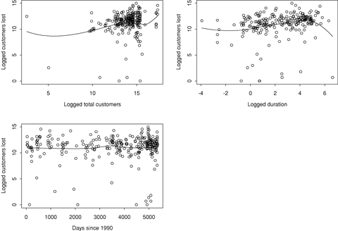
Plots of logged customers lost versus event characteristics in the United States with loess lines superimposed on plots.
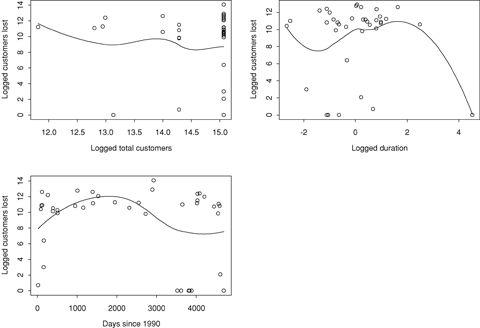
Plots of logged customers lost versus event characteristics in Canada with loess lines superimposed on plots.
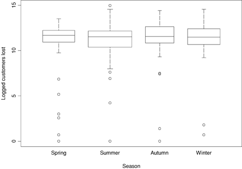
Side-by-side boxplots of logged customers lost separated by season, U.S. data.
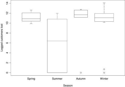
Side-by-side boxplots of logged customers lost separated by season, Canada data.
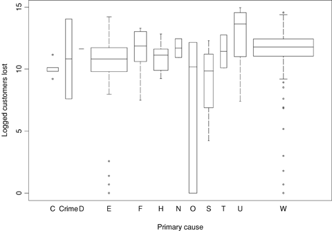
Side-by-side boxplots of logged customers lost separated by primary cause, U.S. data.
Note: See Table I for the definitions for primary cause.
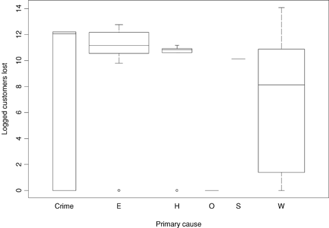
Side-by-side boxplots of logged customers lost separated by primary cause, Canada data.
Note: See Table I for the definitions for primary cause.
The primary important predictors of customers lost in the U.S. data are total number of customers served by a utility and primary cause. A 1% increase in total customers is associated with a 0.18% estimated increase in customers lost, holding all else in the model fixed. In contrast, in Canada, having more customers served is associated with having fewer customers lost, although the relationship is very weak (and not close to statistical significance). The relationships between customers lost and duration are not significantly different in the two data sets, with a joint estimate implying that a 1% increase in duration is associated with a 0.2% increase in customer loss. Further, while there is no evidence of a time trend in customer loss in the U.S. data, in the Canada data, given the other predictors, customer loss is decreasing at an estimated 29.5% annual rate.
Customer losses are higher for natural disaster, crime, unknown causes, and third party, and lower for system protection, capacity shortage, and equipment failure, holding all else in the model fixed. It is interesting to note that the largest customer losses are coming from causes that are clearly beyond the control of the utility, while the smallest losses are coming from causes that are internal to the utility, perhaps suggesting that oversight and preparation at the plant level can be effective in reducing the effects of incidents. In the Canada data, there is also a primary cause effect with equipment failure, human error, and system protection having generally higher customer losses, and crime and weather having smaller losses. The boxplots shown in 5-8 were constructed so that the width of the box is proportional to the square root of the sample size for that group, so the wider the box, the more information there is for that group. It is evident that most incidents are either weather related or due to equipment failure, so effects related to these causes have the largest practical effect on the public. There is little evidence of a seasonal effect in the U.S. model, whereas in the Canada model a marginally significant season effect is that fewer customers are lost during the summer.
Table III summarizes the differences between the two countries with respect to the model in terms of the relationship with the number of customers lost, given that it is nonzero.
| Effect | United States | Canada |
|---|---|---|
| Logged total customers | (Weak) direct relationship | Inverse relationship |
| Time (days since 1990) | No relationship | Inverse relationship |
| Season | No relationships | Customer loss lower in spring and summer |
| Primary cause | Weak relationship, other than crime having higher values | Equipment failure and human error have higher values |
The incident-level analyses reinforce that the seriousness of the outcomes of incidents in Canada has been decreasing over time, while it has been increasing or staying the same in the United States. The earlier arguments about potential reasons why the number of more serious incidents has not been growing in Canada apply here as well: the geographic distribution of the incidents in Canada is changing over time, Canadian hydroelectric power plants have more experience with long-distance power transfers than do U.S. plants, and electricity demand in Canada is growing at a slower rate than in the United States.
4.2.2. Duration of an Outage
The observed relationships for duration of an outage are described in 9-14 for the U.S. and Canada data.
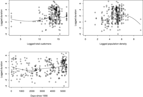
Plots of logged duration versus event characteristics, U.S. data.
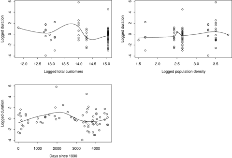
Plots of logged duration versus event characteristics, Canada data.
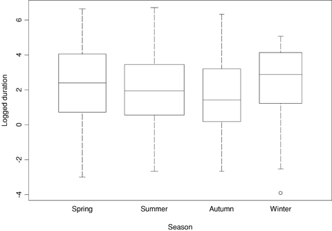
Side-by-side boxplots of logged duration separated by season, U.S. data.
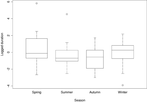
Side-by-side boxplots of logged duration separated by season, Canada data.
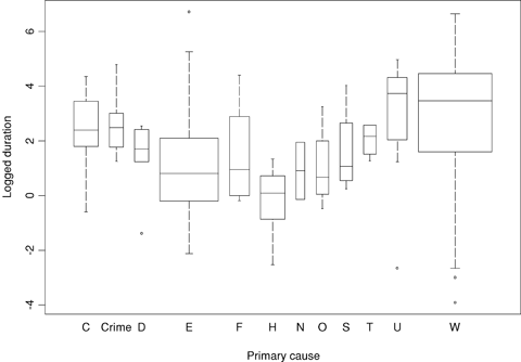
Side-by-side boxplots of logged duration separated by primary cause, U.S. data.
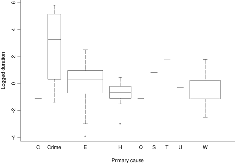
Side-by-side boxplots of logged duration separated by primary cause, Canada data.
As Figs. 9 and 10 show, there is little evidence of a relationship between logged duration and logged total customers served by an affected utility. There is evidence of a positive relationship with logged state population density (ignoring the two relatively short events at the very high population density level in Fig. 9). There is weak evidence of the time trend on duration in the United States, but little evidence in Canada. There is some evidence of a season effect, with winter and spring events longer and autumn and summer events shorter in both countries. There is a clear relationship with primary cause of an outage. In the U.S. data, the two most common causes, equipment failure and weather, are very different, with the former associated with shorter events and the latter associated with longer ones. In the Canada data, crime has noticeably longer incidents than the other causes. Overall, incidents are much shorter in Canada than they are in the U.S.; the median duration in the U.S. (7.7 hours) is almost ten times that in Canada (0.8 hours).
The results of the WLS model for the U.S. data imply that a 1% increase in population density is associated with a 0.33% increase in duration, holding all else in the model fixed. The season effect is that, holding all else in the model fixed, winter events have expected duration that is 2.25 times the duration of summer events, with autumn and spring in between. Presumably, this has something to do with issues such as the difficulty in traveling to downed power lines in snow and ice.
Holding all else fixed in the U.S. model, incidents caused by human error, natural disaster, demand reduction, and equipment failure tend to be shorter, while those caused by system protection, third-party, weather, and unknown causes tend to be longer. Considering that more than ¾th of the events are caused by equipment failure or weather, the contrast between the two is particularly important (events caused by weather are expected to last more than five times longer than those caused by equipment failure, holding all else in the model fixed).
The pattern of durations over time in the U.S. model is worth further comment. A regression of logged duration on time alone implies an estimated 11.6% annual increase in duration. Figure 15 shows a loess curve for the estimated expected duration using these incident-level data. Up until 1994, durations were getting shorter. This turned around in 1995, and for a few years the average duration went up 15–25% annually. This was followed by a long period (1998–2001) of fairly stable growth of 10–20%. Finally, from 2002 onward, average durations have started increasing again at a high 30–40% rate. Thus, the constant estimate of 11.6% annually obtained from the regression model actually seems to mask some very different periods in average duration change.
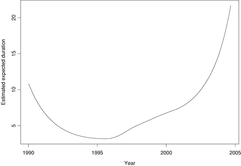
Loess curve for estimated expected duration over time.
The time variable is still highly significant even if season, population density, and total number of customers are added as predictors. However, when primary cause is added, its significance disappears, which shows that it is the primary cause effect that is driving the apparent time trend effect.
Recall that more than three-fourths of the incidents are either equipment failure or weather related, and that incidents caused by equipment failure tend to be shorter, while weather-related ones tend to be longer. In fact, weather-related incidents are becoming more common, while equipment-failure-related ones are becoming less common, and this accounts for much of the overall pattern of increasing average durations by season. Since the mid 1990s, relatively speaking, equipment failures are going down and weather incidents are going up, while before that the opposite pattern was occurring. This corresponds exactly to the drop in durations up to 1995, and the increase since then noted earlier. Thus, it would seem that further study of why equipment failures are becoming less common (relatively speaking) and weather-related events are becoming more common is warranted. At least part of the latter pattern is probably not related to the power grid at all. On the basis of the data from U.S. Department of Homeland Security (2006), officially declared federal disasters have been increasing at a rate of roughly 2.8% annually since the 1950s; most of those are weather related (flooding, hurricanes and tropical storms, tornadoes, winter storms), so an increase in weather-related outages is not surprising (although this would not explain why weather-related outages were dropping before the mid 1990s).
Unlike the U.S. model, the Canadian model for duration shows little evidence of any relationships at all. The primary cause effect is damped down because while crime apparently has longer incidents, that cause also had more variability in durations. A simplified version of the model with only cause and season suggests that each effect is only weakly significant. The season effect implies that, holding all else in the model fixed, winter and spring events have an expected duration that is roughly 2.5 times the duration of autumn events. The adjusted means for primary cause show that, holding all else fixed, incidents caused by crime tend to be longer.
5. PREDICTING OUTAGE OUTCOMES
The models described in the previous section provide useful information about the factors related to the seriousness of a power outage. These results can also be used to construct predictions for outage outcomes based on different scenarios, and thereby provide probabilistic assessments of the risks associated with these events. By examining predicted duration and customer loss under different conditions, it is possible to map out possible outage outcomes. One application of these results is to predict outcomes of potential terrorist attacks on the electric grid. Although there are no data on such attacks for the United States or Canada, expert panels may be able to determine what causes are likely to be similar to those of a terrorist attack. Hence, scenarios that predict the outcome of such attacks in terms of numbers of customers lost and duration of an outage can be constructed. These outage characteristics can then be used to estimate economic costs associated with business losses for a geographical area such as a city. The models allow the user to predict outage characteristics for a city such as New York, for example, by including properties such as state population density and the number of customers served by the local utility. In addition, differences in outcomes based on the season of a potential terrorist attack can also be included in a scenario.
In this section, we construct scenarios for cities with characteristics like those of New York and Toronto. These two cities provide an interesting contrast, since they are not only from different countries, but the structure of the city power grid is noticeably different: New York has relatively few transmission lines, while Toronto has many. Using the characteristics of the utilities in these cities, the estimated duration of an incident, separated by season and cause, is determined for each city using the weighted least squares model described in the previous sections. Since (logged) duration is an important predictor for customer loss, these estimated durations are then used as inputs to the logistic regression model discussed to estimate the probability that there is zero customer loss. Finally, the estimated (logged) duration value, along with the characteristics of the utility, are used to estimate the number of customers lost, given there is nonzero customer loss, using the weighted least squares model.
In addition to estimated expected values, these methods allow us to construct 50% prediction intervals for duration and for customer loss (given that the loss is nonzero) for any cause and season for the two cities. These intervals give the central range within which there is 50% chance of the duration or customer loss falling in an individual incident.
5.1. Duration of an Incident
First, consider intervals for duration. Fig. 16 shows 50% prediction intervals for the duration of an incident in New York City in the summer. The horizontal tick on each line is the estimated expected duration for a summer New York City outage with that cause, while the vertical line gives the 50% prediction interval. The figure shows that the cause of the incident is related to both the level of duration (e.g., human error and demand reduction are associated with shorter incidents and weather and unknown cause are associated with longer ones) and the variability in duration (e.g., third-party cause and system protection have similar expected durations, but durations of incidents caused by system protection are much more variable).
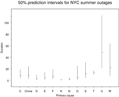
Prediction intervals for duration of summer outages in New York City.
Figure 17 shows intervals for New York City outages during the winter separated by cause. The pattern of relative estimates and prediction intervals is the same as for the summer incidents, but the averages and intervals are shifted up by a factor of two, reflecting that outages are longer on average during the winter.
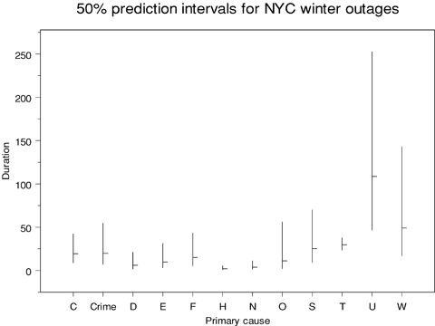
Prediction intervals for duration of winter outages in New York City.
Table IV summarizes the estimated expected durations (in hours) for New York City scenarios.
| Spring | Summer | Autumn | Winter | |
|---|---|---|---|---|
| Capacity shortage | 12.5 | 8.5 | 11.9 | 19.2 |
| Crime | 12.8 | 8.7 | 12.2 | 19.6 |
| Demand reduction | 3.9 | 2.7 | 3.7 | 6.0 |
| Equipment failure | 6.3 | 4.3 | 6.0 | 9.7 |
| Fire | 9.8 | 6.7 | 9.3 | 15.0 |
| Human error | 1.3 | 0.9 | 1.3 | 2.0 |
| Natural disaster | 2.5 | 1.7 | 2.4 | 3.8 |
| Operational error | 7.2 | 4.9 | 6.8 | 11.0 |
| System protection | 16.4 | 11.2 | 15.5 | 25.1 |
| Third party | 19.4 | 13.2 | 18.4 | 29.7 |
| Unknown | 70.7 | 48.3 | 67.2 | 108.5 |
| Weather | 32.0 | 21.8 | 30.4 | 49.1 |
Fig. 18 shows corresponding 50% prediction intervals for the duration of an incident in Toronto in the summer. It is apparent that predicted durations are similar (and relatively short) for all causes other than crime; for crime-related incidents both the expected duration and its variability are high, yielding a wide prediction interval.
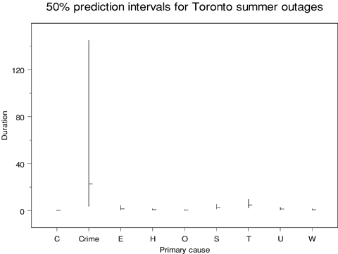
Prediction intervals for duration of summer outages in Toronto.
Fig. 19 shows intervals for Toronto outages during the winter by cause. The pattern of relative estimates and prediction intervals is the same as for the summer incidents, but the averages and intervals are shifted up by roughly 40%, reflecting that outages are longer on average during the winter.
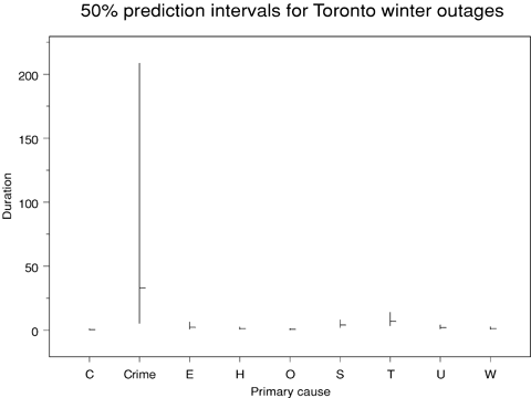
Prediction intervals for duration of winter outages in Toronto.
Table V summarizes the estimated expected durations (in hours) for Toronto scenarios.
| Spring | Summer | Autumn | Winter | |
|---|---|---|---|---|
| Capacity shortage | 0.4 | 0.3 | 0.2 | 0.5 |
| Crime | 26.2 | 22.9 | 12.7 | 33.0 |
| Equipment failure | 1.8 | 1.5 | 0.9 | 2.2 |
| Human error | 1.0 | 0.9 | 0.5 | 1.3 |
| Operational error | 0.5 | 0.4 | 0.2 | 0.6 |
| System protection | 3.2 | 2.8 | 1.5 | 4.0 |
| Third party | 5.5 | 4.8 | 2.6 | 6.9 |
| Unknown | 1.6 | 1.4 | 0.8 | 2.0 |
| Weather | 1.0 | 0.8 | 0.5 | 1.2 |
5.2. Customer Loss of an Incident, Given that it is Nonzero
Using the estimated durations as inputs for the model, prediction intervals for customer loss (given that the loss is nonzero) can also be constructed. These are useful in assessing the economic impact of an outage, although this is only a crude approximation, given the differing economic impacts of an outage for different classes of customers. The intervals for a city with characteristics like those of New York City are shown in Figs. 20 and 21. Once again there are considerable differences in both level and variability depending on the cause of the incident. The intervals for winter outages are centered at higher values, but this is an indirect, rather than direct, effect: while there is little difference in expected customer loss for summer and winter given the other predictors, outages are longer on average during the winter than during the summer, and longer outages are associated with more customers being affected.
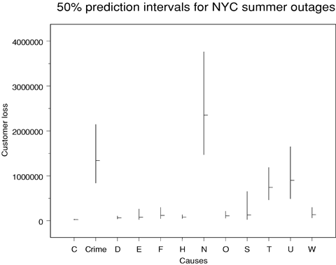
Prediction intervals for customer loss (given that it is nonzero) of summer outages in New York City.
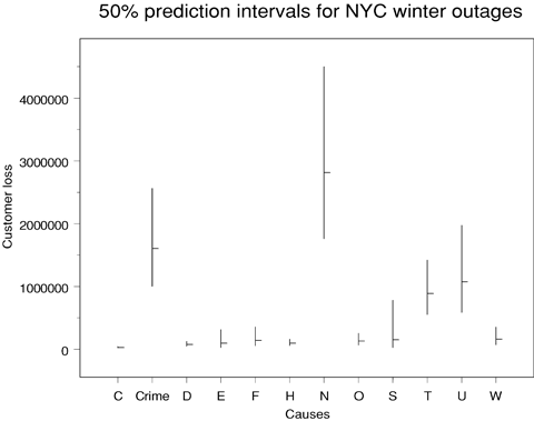
Prediction intervals for customer loss (given that it is nonzero) of winter outages in New York City.
Two values are needed to estimate the number of customers lost in an outage: the estimated probability that an incident will have zero customer loss and the expected customer loss given that it is nonzero. Table VI gives estimated probabilities of zero customer loss for New York City outages.
| Spring | Summer | Autumn | Winter | |
|---|---|---|---|---|
| Capacity shortage | 0.056 | 0.028 | 0.049 | 0.052 |
| Crime | 0.464 | 0.300 | 0.431 | 0.447 |
| Demand reduction | 0.575 | 0.401 | 0.542 | 0.558 |
| Equipment failure | 0.053 | 0.027 | 0.047 | 0.050 |
| Fire | 0.054 | 0.027 | 0.047 | 0.050 |
| Human error | 0.066 | 0.034 | 0.059 | 0.062 |
| Natural disaster | 0.132 | 0.070 | 0.117 | 0.124 |
| Operational error | 0.022 | 0.011 | 0.019 | 0.020 |
| System protection | 0.000 | 0.000 | 0.000 | 0.000 |
| Third party | 0.519 | 0.348 | 0.485 | 0.502 |
| Unknown | 0.039 | 0.019 | 0.034 | 0.036 |
| Weather | 0.008 | 0.004 | 0.007 | 0.007 |
Table VII provides the estimated expected customer losses (given nonzero customer loss) for New York City scenarios.
| Spring | Summer | Autumn | Winter | |
|---|---|---|---|---|
| Capacity shortage | 42,984 | 25,448 | 31,998 | 30,434 |
| Crime | 2,265,524 | 1,341,245 | 1,686,511 | 1,604,029 |
| Demand reduction | 110,022 | 65,136 | 81,903 | 77,897 |
| Equipment failure | 135,641 | 80,302 | 100,974 | 96,036 |
| Fire | 200,667 | 118,800 | 149,381 | 142,076 |
| Human error | 137,347 | 81,313 | 102,244 | 97,244 |
| Natural disaster | 3,975,563 | 2,353,628 | 2,959,504 | 2,814,765 |
| Operational error | 186,627 | 110,488 | 138,930 | 132,135 |
| System protection | 216,197 | 127,994 | 160,942 | 153,071 |
| Third party | 1,255,536 | 743,308 | 934,651 | 888,941 |
| Unknown | 1,519,551 | 899,611 | 1,131,190 | 1,075,867 |
| Weather | 228,837 | 135,477 | 170,352 | 162,021 |


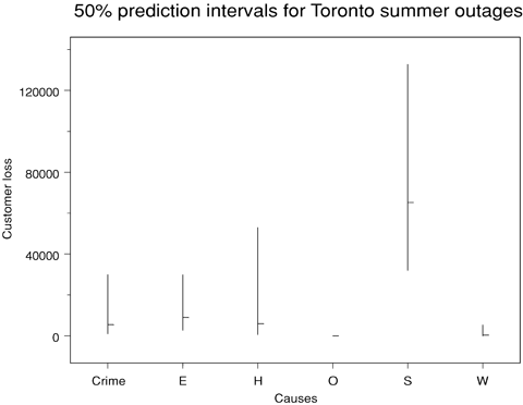
Prediction intervals for customer loss (given that it is nonzero) of summer outages in Toronto.
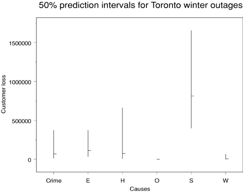
Prediction intervals for customer loss (given that it is nonzero) of winter outages in Toronto.
Table VIII gives estimated probabilities of zero customer loss for Toronto outages.
| Spring | Summer | Autumn | Winter | |
|---|---|---|---|---|
| Capacity shortage | 1.000 | 1.000 | 1.000 | 1.000 |
| Crime | 0.806 | 0.996 | 0.986 | 0.971 |
| Equipment failure | 0.525 | 0.987 | 0.948 | 0.898 |
| Human error | 0.806 | 0.996 | 0.986 | 0.971 |
| Operational error | 0.000 | 0.000 | 0.000 | 0.000 |
| System protection | 0.000 | 0.003 | 0.001 | 0.000 |
| Third party | 1.000 | 1.000 | 1.000 | 1.000 |
| Weather | 0.986 | 1.000 | 0.999 | 0.998 |
Table IX provides the estimated expected customer losses (given nonzero customer loss) for Toronto scenarios.
| Autumn | Spring | Summer | Winter | |
|---|---|---|---|---|
| Crime | 241,937 | 39,187 | 5,451 | 67,909 |
| Equipment failure | 399,752 | 64,748 | 9,006 | 112,205 |
| Human error | 263,445 | 42,670 | 5,935 | 73,945 |
| Operational error | 7 | 1 | 0 | 2 |
| System protection | 2,896,406 | 469,131 | 65,256 | 812,982 |
| Weather | 16,419 | 2,659 | 370 | 4,609 |

6. CONCLUSIONS
A critical need exists to develop the means to provide decision tools to estimate the consequences of terrorist attacks against electric power systems as part of the growing field of risk analysis for terrorism events. This is particularly difficult in the United States given the very few terrorist attacks that have disabled electric power systems, and none that have actually directly targeted electric power. This article has provided a framework for analyzing available electrical outage data to gain a better understanding of the factors that influence outcomes, such as the number of customers lost and duration of an outage. The statistical models used reinforce the importance of probabilistic assessment of risk, whether that is estimating the probability of zero customer loss, or constructing prediction intervals within which outage characteristics such as duration and customer loss are predicted to fall with specified probability. Clearly, such risk assessment also leads directly to issues of risk management, such as in questions of resource allocation.
The analyses were done for the United States and Canada and the results show how the models can be used to identify important differences for the two countries. These patterns, besides being of interest in and of themselves, highlight the need for general statistical models for probabilistic risk assessment, since it is apparent that the consequences of outages differ for incidents in different places, at different times, and with different underlying characteristics.
First, at the level of overall trends in events over time, the number of disturbances to the electric grid increased over the period studied for both countries. In the United States, the annual rate of increase was estimated to be 7.2% and in Canada it was 8.2%. However, while the number of events with nonzero megawatt loss increased in the United States at an annual rate of 10%, in Canada there was no evidence of a time trend for these events. Similarly, the number of events with nonzero customer loss increased in the United States at an estimated annual rate of 14% but in Canada the model provided little evidence of any relationship with season or time for these events.
Second, the results of the event-level analyses can provide insights into the dynamics underlying the factors affecting disturbances in each country. The results show that the dynamic is different in the two countries. For example, in estimating the number of customers lost during an outage, the model predicts that in the United States there is a weak but direct relationship with total number of customers served by a utility. In Canada, the model suggests an inverse relationship. In the U.S. model, there is no relationship between customer loss and season, whereas in the Canada model customer loss is lower in the spring and summer. In modeling the duration of an event, the results suggest that in the United States, outage duration was decreasing in the early 1990s and then started to increase in the mid-1990s. This is due to the fact that the relative frequency of the cause of the events changed over time, with weather-related events becoming more common over time during this period and equipment-related disturbances less so. Weather-related events are associated with longer durations. The Canada data, on the other hand, show little evidence of any relationships.
Third, the results of these models can provide information about outcomes such as expected customer loss and duration of outages in different seasons and for cities with different characteristics, and hence inform response to outages in both terror-related and nonterror-related circumstances. The results of the 50% prediction intervals shown in this article for cities with characteristics like those of New York City and Toronto are very different. For example, in terms of outage duration, the results for New York City suggest that the longest durations are to be expected from weather events, unknown causes, and third parties. In Toronto, the highest expected durations are from crime-related events. In terms of customer loss, the results for New York City suggest crime and natural disasters could have the biggest impact. In Toronto system protection, equipment failure, human error, and crime have the highest impact.
These kinds of scenarios can be used as inputs into risk management policies. The incident analysis based on statistical regression modeling presented in this article can be used to provide inputs into economic valuation frameworks to estimate the potential impact of a terrorist attack or a natural hazard on the electricity infrastructure. Some of the causes associated with electric outages are more likely to be similar to the impact of a terrorist attack than others. The results of these models can then be used to estimate potential economic costs, such as business losses, associated with a terrorist attack. The advantage of the model presented in this article for such purposes is that it can be used for quick estimates and assessments (Zimmerman et al., 2005, 2007), although it should be noted that such estimates could be considered worst-case scenarios, since they would not reflect adaptive behavior of customers. This methodology can also complement other frameworks of analysis such as input-output analysis (I-O) (Rose et al., 1997; Rose & Benavides, 1998; Haimes et al., 2005; Gordon et al., 2005) and computable general equilibrium (CGE) models (Rose & Liao, 2005) that have also been applied to estimate the economic impacts of natural disasters or terrorist events.
The data can be modified or tailored for specific areas and season. Understanding the differences between the factors affecting outages in Canada and the United States is also important because the electricity grids of both countries are interdependent. For example, between 1982 and 2002, U.S. annual imports of electricity from Canada generally ranged between 20 and 50 billion kilowatthours (U.S. Department of Energy, 2005). Hence, outages in one country can have important impacts on the other. The differences in the patterns in the United States and Canada also have implications for outage patterns in the future, as interdependencies grow between the two countries.
The regression models discussed in this article could be improved if more precise data were available. Examples of potential improvements include using temperature on the day of the outage instead of season and a better proxy for local population density. It is important to note that the data on electric disturbances are collected by NERC on a voluntary basis. Utilities are not required to provide this information. In addition, it is not possible to know if the way the data are reported has been consistent over time. In conducting studies of events over time in the electricity sector an important factor affecting causes and outcomes is changes in the regulatory environment under which utilities operate. Including these changes in the regression models could be a future research direction in this field. In addition, it is important for more detail to be included in future reports about outage incidents in order to link causes of outages more closely to terrorist attack circumstances.
ACKNOWLEDGMENTS AND DISCLAIMER
This research was supported by the U.S. Department of Homeland Security through the Center for Risk and Economic Analysis of Terrorism Events (CREATE), Grant EMW-2004-GR-0112. However, any opinions, findings, and conclusions or recommendations in this document are those of the author(s) and do not necessarily reflect views of the U.S. Department of Homeland Security. The authors wish to thank graduate research assistants Nicole Dooskin, Ray Hartwell, and Justin Miller and assistant Wendy Remington for their help in assembling the database. The authors also wish to acknowledge the very helpful suggestions of the anonymous reviewers.


