Cost-efficient equitable water distribution in Algeria: a bicriteria fair division problem with network constraints

1. Introduction

This paper presents a real water distribution case in a rural area within the region of Kabylia, Algeria, supported by the Spanish Cooperation and Development Agency. At first, it may be described as a relatively standard water distribution problem, with water coming from various wells, several intermediate water deposits and pumping stations, and consumption taking place in villages, with very disperse population. However, especially in the summer, when less water is available and population almost doubles, there is considerable water scarcity, aggravated by significant water losses in the network. Unfortunately, the current management system in place seems to privilege some villages, in that lack of water tends to affect specific villages for too long periods of time. This has caused political unrest. A second contextual feature of interest stems from the cultural traditions in the region. Traditionally, Kabylians have preferred to live up in the mountains, and this creates important engineering and economic problems, with a very high proportion of water distribution costs spent in electricity consumption for pumping the water.

In Udías et al. (2011), we performed a preliminary detailed data and design analysis of the current distribution network to understand the faults in its current operation. The inclusion of new pipes, the tank sizes and locations, and the pump operational schedules were considered as design variables. We essentially concluded that the incumbent problem was not one of water availability, as believed by our client, but it was actually produced mainly by water losses, including water thefts, and inappropriate distribution schedules. Thus, unless willing to introduce important infrastructure investments, there was a need to distribute water in a much more equitable and economical fashion. We tackle both issues in this paper. We initially dealt with this bicriteria problem in two phases, assuming a lexicographic approach (see, e.g., Yu et al., 1985), as the first objective (maximize equity) seemed much more important to our client than the second one (minimize cost). Note that, as usual with water systems (see, e.g., de Neufville et al., 1971; Ríos Insua and Salewicz, 1995; Walski et al., 1987), we face a multiobjective problem.

Therefore, in a first stage, we aimed at determining an equitable water distribution schedule for the region, taking into account various distribution constraints. For whatever reason, equity is in the eye of the beholder. Indeed, our initial aim was to implement the objective function required by the water distributors, which reflected the need that all inhabitants would receive the same volume of water. However, upon reflection, we realized that we could implement several other objective functions encapsulating equity, many of them available from the bargaining literature (see, e.g., Raiffa et al., 2007), although some of the equity related objective functions are new. The problem may be viewed, thus, as a fair division problem with network constraints: we need to divide a good fairly, the water available over a period of time, and distribute it efficiently. (See Brams and Taylor, 1996, for an introduction to fair division problems.) There are also connections with the bankruptcy problem (see Aumann and Maschler, 1985), although we need to operate over time and with network constraints, as novelties in our approach.

Once we have obtained a fair scheme, which is, we insist, the most important objective for the management, we try to implement it in the less-costly way, taking into account the time-varying costs of pumping water, due to the changes in electricity tariffs, according to a daily schedule. This problem may be formulated through a mixed linear-integer optimization model. Then, by varying the minimum equity level acceptable and finding the corresponding cheapest distribution schedule, we are able to generate the Pareto water distributions schemes. In this way, the management may understand the tradeoffs between the total pumping cost and the satisfaction of water demand, and make decisions accordingly.

The structure of the paper is as follows. First, we formulate in Section 2. the problem as presented by the water company, with an objective function aimed at providing the same amount of water to each inhabitant. We then provide a discussion of several other potential objective functions, which might be used to obtain equitable water distribution schedules, and discuss them. Once we have chosen our equitable schedule, we discuss in Section 3. how to distribute it in the least costly manner and how to generate Pareto-efficient schedules that improve upon the lexicographic schedules identified and facilitate a powerful management tool to the water distributor. We illustrate the methodology in Section 4. with our motivating case referring to the region of Kabylia, presenting the results of our analysis. We end up with some discussion.

2. Equitable water distribution

Water distribution problems may be described in relatively simple terms (see, e.g., Soncini-Sessa et al., 2007). We have a number of water sources, usually wells and reservoirs, which together provide the water offered. We also have a number of water consumption points, which, depending on the granularity of the problem, might refer to houses or villages. We aim at satisfying their water demand, taking into account a number of physical and engineering constraints, reflecting the structure of the distribution network, typically including intermediate deposits and pumping stations. Figure 1 provides a simple scheme to which we shall refer later in the article, which reflects the structure of the problem used in Section 4., just with wells as source points and deposits as intermediate points.

It could be the case that, given the water distribution network features, we are not able to satisfy completely the demand. We, thus, look for ways of making this unsatisfied demand as balanced as possible among consumers. We call this problem “equitable water distribution.” We formulate it as follows.

2.1. Decision variables and constraints

We shall consider the operation of a water distribution system over a time T. The operating time will be designated t, with . Assume there are source points, designated by ; intermediate points, designated by ; consumption points, designated by ; well pumps (pumping water from the source point i to the network), designated by ; and, finally, station pumps (pumping water from the initial pump station j to the deposits), designated by . At each time t:

• We define integer variables and to describe the state of the pumps,
  
  and, similarly, for .
• We decide to extract a volume of water from the ith source point, with , where is the maximum water extraction capacity from the ith source point at time t.
• The water stored at the jth intermediate point is , with , where is the maximum water storage at j. We should, however, be careful as we could be tempted to extract too much water from the deposits, rendering them impossible to be refilled for the next period. We must ensure that jeopardizing future supplies, in exchange for short-term gains, will not occur. To do so, we impose an operational constraint on each deposit, actually requiring them to have a minimum prescribed water level at the beginning of each period, leading to the constraint
  (1)
• We decide to derive a volume of water from the ith source point toward the jth intermediate point, with
  (2)
  where is the maximum water flow capacity for the conduction between the source point i and the intermediate point j. Clearly,
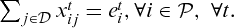
• The capacities of the well pumps do not vary with time. Thus, the following condition must hold
  (3)
  indicating that the water pumped from the ith well cannot exceed the incumbent maximum water capacity.
• We decide to release a volume of water from the intermediate point j toward the intermediate point , with
  (4)
  where is the maximum water flow capacity between j and .
• The capacities of the station pumps do not vary with time. Thus, the following condition must hold:
  (5)
• We decide to release a volume of water from the intermediate point j to the consumption point k, with
  (6)
  where is the maximum water flow capacity for the conduction between j and k.
• The consumption point k will demand a volume of water, which will be assumed known in this paper.

For the sake of generality, we have described a fully connected distribution network with links between all intermediate points; links between each source point and every intermediate point and, finally, links between each intermediate point and every consumption point. Links that are not feasible may be described through a zero upper bound on the water capacity flow.

The following additional constraints will hold in our problem:

• Mass continuity conditions for intermediate points, describing that the variation in water stored at the jth intermediate point between times and t equals the balance between the inflows coming from source points and the releases toward consumption points
  (7)
• Demand satisfied at each consumption point. We aim at achieving the target demand . For this, we introduce slacks
  (8)
  where represent, respectively, the water surplus and deficit at consumption point k and time t. Both slacks cannot be positive simultaneously. To achieve this, we may introduce the constraint , although this constraint may be removed, depending on the objective function introduced.

A distribution schedule will be defined through the vector

We shall denote all of the above constraints through , defining all feasible distributions schedules.

2.2. Objective function

We describe now various potential objective functions referring to equity in water distribution. We shall start by considering the objective function originally proposed by the incumbent water distribution company and, then, several alternatives. Implicitly, we shall assume that, for each village, the utility it attains with a water distribution schedule coincides with minus the per capita water deficit inflicted. Each village aims at minimizing its per capita water deficit and, collectively, we aim at balancing such deficit, based on one of the following possibilities.

Egalitarian solution

The initial objective function suggested by the water distribution company aimed at inflicting the same water deficit to all inhabitants and minimizing such deficit. The deficit for the kth consumption point over the whole planning period is . If is the population of the kth consumption point, the per capita water deficit is . As required by the water distribution company, we would aim at solving

(9)

This corresponds to an egalitarian solution in arbitration (see, e.g., Raiffa et al., 2007). Making such analogy lead us to think about considering alternative arbitration solution concepts.

Smorodinsky–Kalai solution

A first alternative concept is the Smorondinsky–Kalai solution (see, e.g., Kalai, 1977, or Alexander, 1992). In our context, we formulate it as the minmax problem

We may reformulate it through

(10)

Nash solution

Another important solution concept is Nash cooperative equilibria (see, e.g., Nydegger and Owen, 1974; Alexander and Ledermann, 1994; Mariotti, 1999). In our context, as represents a loss, we multiply it by −1, and add up a constant to make it nonnegative (and account for the disagreement point). In that case, we would have to solve the problem

Equivalently, we could solve

(11)

Utilitarian solution

Finally, a fourth important arbitration concept is the utilitarian one (see Ponsati and Watson, 1997), which aims at maximizing the sum of attained utilities (in this case, minimizing the sum of deficits)

Equivalently, we would aim at maximizing the average utility, i.e., minimizing the average water deficit inflicted at the consumption points

(12)

Standard deviation solution

Additionally, though not usually included as an arbitration solution, we could aim at minimizing the standard deviation of the water deficits to the villages. Thus, we would be solving the problem:

(13)

2.3. Inter- and intraequity

The above approaches provide distribution schedules that aim at reflecting equity among consumption points, providing a global view of the distribution problem over the period T. However, it could be the case that deficits among villages are balanced, i.e., deficits among consumers are reasonably similar across all the region, but the deficit for at least one of the consumers is unbalanced over time. As an example, for a given consumption point k, the per capita water deficits would be

which compared with the values received by other consumption points might seem equitable. However, it could be the case that the above quantities are very unequal, thus leaving the consumption point with little water for some time periods, with much bigger volumes of water for others. Therefore, we need to consider both the intervariability, defined above through , and the intravariability, defined as:

Then, we could aim at maximizing the water delivered, or minimizing the deficit, and minimizing both the intra- and intervariability, by considering the problem

for appropriate weights reflecting the importance given to various objectives.

3. Cost-effective equitable water distribution

We have described various models leading to equitable distribution schedules in that they minimize deficits in a balanced way among consumers over time. Once we have chosen a distribution schedule, we discuss how to distribute water in the most cost-effective manner, taking into account that pumping costs vary according to a daily schedule. This issue is specially important in our incumbent case study, as pumping costs constitute the largest share of distribution costs.

To do so, we divide a given period t in m parts. We assume that, at the lth part of the period, the distribution costs are . The schedule at a given period t is , which decomposed over the m points will be expressed as

At each period t, we aim at minimizing the total pumping costs

subject to constraints

, together with the constraints in relation with maximum storage, maximum pumping capacities, and continuity conditions, mentioned above. Specifically, conditions 1–8 must hold at each time subperiod. Solving this optimization problem provides the cheapest pumping schedule fulfilling the equity requirements.

The above approach is lexicographic, see e.g., Yu et al. (1985), in that the equity objective is much more important than the cost objective, as suggested by our client. However, in order to further explore the tradeoffs between both objectives, we shall consider the full biobjective problem as follows. To each feasible distribution schedule, , we associate its cost (to be minimized), and its equity (to be maximized). The biobjective problem we face is, then,

For this problem, would be a Pareto-optimal distribution schedule if there is no other such that and .

We shall approximate the set of Pareto-distribution schedules through an ε-constraint approach: we first adjust the minimum acceptable level of the equity measure, find the corresponding most equitable schedule, and, then, the least expensive implementation of such schedule. By varying parametrically the minimum acceptable equity level, we may approximate the whole Pareto set, see e.g., Yu et al. (1985). As an example, if we consider the Smorodinsky–Kalai concept to measure equity, we would solve for several the problem

which would provide an optimal schedule with equity level , which would in turn lead to the optimal cost . The use of such Pareto frontier is a powerful management tool for the water distributor in that, for a given distribution cost, the company may find the most equitable distribution schedule, and, vice versa, for a given equity level, they may find the least costly schedule.

4. Case study: cost-efficient equitable water distribution in Kabylia

Kabylia is located in the North East of Algeria, bounded in the North by the Mediterranean Sea, in the East by the region of Bedjaia, in the West by the region of Boumerdes, and in the South by the region of Bouira. The total area of the region is 2,957 km², 80% of which lies on slopes with inclinations greater than 12%. It is composed of 67 municipalities (1,380 villages) with a total population of more than 1.1 million people.

We have developed a model for a portion of the distribution network in Kabylia, the so-called “Chaine de Tassadort” area, with 110,000 people living in 90 villages. Most of the population is located in mountainous areas with altitudes over 900 m in some cases. The average annual rainfall is around 900 mm/m². The company L'Algerienne des Eaux (ADE) supplies water in the region. In 2009 the reported volume of water supplied amounted to 6,500,559 m³, but only 1,696,294 m³ was billed, a huge loss which resulted in significant shortfalls for the company. These losses are mainly due to leakages and outdated pipes and components in the networks and also due to water thefts. Figure 2 shows the general layout of the Tassadort water distribution network. We have used a special dashed arrow for the connection Tassadort-Mezdata, as it will play an important role in our study. Given the current distribution system and the scarcity of water, it is frequently the case that several villages end up having no water for an extended period, say of a week, specially over the summer. This creates many inconveniences, including the need to transport water by truck to certain villages, social unrest, etc.

The network includes 38 deposits with a total storage capacity of 28,000 m³, six pumping stations with 22 fixed-rate pumps and a total pumping capacity of 5,400 m³ per hour. The main network of pipes spreads over several hundreds of kilometers. The daily average consumption is, approximately, 19,000 m³. The peak demand within a 1-h period is estimated to be around 6% of the daily global demand.

4.1. Outline of methodology used

The choice of the time-step used in the optimization problem is crucial for the computational burden of the problem. The optimization period is denoted by T, and we have discretized it into n steps. Different step lengths may be considered, but we have found a time-step of 1 h to be a reasonable choice, as a trade-off between what would be desirable in real-time scheduling and the need of completing computations before the next update.

While it is possible to envisage an operating horizon longer than 24 h in those places where storage is exceptionally large, most water-distribution networks operate on a 24-h cycle basis, refilling tanks at night, and pumping water from them during daytime. However, we have set a 48-h simulation period (in springtime) in order to consider two consecutive days with significant variations in demand (with an average demand of 150 L per day per person), assuming losses in the network. This would imply that for every decision variable, e.g., a transportation arc, we have to define 48 additional variables corresponding to the water volume transported at each time period. Smaller step lengths would increase in a prohibitive manner the number of variables and the computational burden, due to the presence of hundreds of integer variables. A total period of 48 h is also a reasonable planning period from a sanitary point of view.

Water demand variations occur on a daily basis. We model it through a demand curve, which plots the percentage of daily per capita demand vs. time (Fig. 3). In our approach, we assume the same daily water demand in every village. Different scenarios were generated varying the water demand and infrastructure available on the network to check for robustness of our solution.

We must also take into account in our problem additional considerations concerning energy tariffs. Table 1 shows the energy costs in Algerian Dinars per kWh (DA/kWh), for each of the time periods in which the energy tariffs are structured (night, flat, peak), and on the specific plant from which the water is pumped (Tassadort or Sebaou). We assume that electricity prices do not vary within the planning time. In this regard, the initial simulation time is set at midnight, when the night energy tariff applies and demand is lower.

Table 1. Pumping cost for different times of day and facilities

Facility tariff	Day period	Cost (DA/kWh)
Tassadort	Night	85.33
Tassadort	Flat	161.47
Tassadort	Peak	726.28
Sebaou	Night	150.53
Sebaou	Flat	150.53
Sebaou	Peak	126.68

In our analysis, as mentioned, we have considered two objectives: one refers to minimizing the total pumping cost, whereas the other refers to maximizing equity, based on some of the equitable solution concepts described in Section 2.2.. We compare various solutions with our equity measures and then provide their optimal cost schedules. All computations were performed on a PC with an Intel Core II Duo T7200 processor, with 2 GHz and 2GB of RAM, under Windows XP. The water network was modeled with the aid of the OPL Studio Library v3.7, using ILOG CPLEX 9.0 as solver.

Our network models comprise around 7,000 variables and 60,000 constraints. Each of the cases considered (corresponding to a point in the Pareto frontier) is the result of a run of the model, lasting around 20 min. However, in hardly any of the Pareto points, the optimizer found the optimal solution within these 20 min. Due to the presence of integer variables, the optimizer would usually need more than 24 h to explore the whole search space to find the optimal solution. But as we checked in practice, the estimated solution obtained after 20 min was generally within 99% of accuracy with respect to the optimal one. We should also mention that due to the discrete nature of the variables and , the results have a stepwise profile, as the pumps have two possible states for each planning period (hours in our case): ON or OFF. Therefore, whenever a pipe changes its status, there is a “jump” in the cost and in the volume of water pumped into the network.

In what follows, we will show only graphical results of three of the solutions discussed in Section 2.2., the egalitarian solution 9, the Smorodinsky–Kalai solution 10, and the utilitarian solution 12. We have plotted in the y-axis the total pumping cost of the proposed solution in DA, whereas the x-axis displays the value of the global water deficit resulting from the different solutions. We have not included results for the Nash solution 11 because of the nonlinear nature of its objective function, which prevented us from implementing it in our solver. However, we were able to simulate its behavior for small-scale subnetworks and limited time horizons by linearizing 11 using the fact that for . We found the value to work well in practice, as it ensured positive values within the logarithm in 11. Under this setting, we virtually obtained the same results than those of the utilitarian solution, although further research would be needed here to incorporate the nonlinear features for the whole network and time horizon. For the same reasons, we have not included the standard deviation nonlinear solution 13, although we have obtained results close to those of the egalitarian solution after linearizing 13, using the fact that , for , within the reduced setting explained above.

We have considered two different scenarios regarding the distribution network losses. The first scenario, H₁, assumes that we can satisfy the demand at all network points. The second scenario, H₂, which is more realistic, allows for unfulfillment of the demand at certain points of the network, due to several reasons, e.g., an insufficient flow capacity of a given pipe. We outline the most relevant results in our experiments for both scenarios below. In particular, we investigate different ways of redistributing water when the available budget is reduced and demand cannot be satisfied at all consumption points.

4.2. Scenario H₁

Figure 4 shows some values of the Pareto frontier for the egalitarian (light gray circles), the Smorodinsky–Kalai (dark gray squares), and the utilitarian (black diamonds) solutions.

• For the utilitarian solution (black diamonds), as the available pumping budget is progressively reduced, the system will stop first supplying water to those points with higher pumping costs. Usually, these are located on top of the hills. If there are several consumption points with the same (expensive) pumping costs, and the budget is further reduced, the system will first cut water supply to those villages with larger population. In this manner, the corresponding term contributing to 12 will be smaller, as it is divided by a larger number, the population at the kth consumption point. We should remark that this solution leads to cutting the water supply to all the inhabitants of a certain village at the same time. This policy is actually quite unfair, although from a purely economic point of view, it is the most advantageous one. For our water network, the first village that would eventually suffer water restrictions is Bouhinoune Haut, which is placed high on the mountains, needs three intermediate pumping facilities (thus notably increasing the pumping costs), and has, approximately, 9,000 dwellings, whereas the average number in the nearby villages is around 1,200.
• For the egalitarian solution (light gray circles), the per capita water deficit is the same for all villages. Thus, when the available pumping budget is reduced, this water scarcity is equally distributed among all the inhabitants of all the villages, regardless of their population size or location. This would be the fairest solution, although it is typically more expensive than the utilitarian one. To gain insight about this phenomenon, we have zoomed in Fig. 5 the central part of Fig. 4. As we can observe, the costs in the utilitarian solution are, on average, around 15% less than those of the egalitarian solution (i.e., with the same available budget, the utilitarian solution supplies 15% more water, but at the expense that those villages with the most expensive pumping costs will not receive water at all). The fact that in Fig. 5 some points apparently break the descending trend of the graphic is reasonable, as we have to keep in mind that what we are plotting in the x-axis is the total water deficit, which is not an objective in itself, but, rather, a mean to compare the different objective functions proposed in Section 2.2..
• For the Smorodinsky–Kalai solution (dark gray squares), the results obtained are similar to those of the egalitarian solution. However, there are subtle differences in the way in which restrictions are managed as the available pumping budget is progressively reduced. With the egalitarian solution, if in a given village the demands are satisfied up to, say, 95%, the same fulfillment will be accomplished for the rest of the villages. If this percentage continues decreasing, it will do so in the same way for all the villages. On the contrary, for the Smorodinsky–Kalai solution, the villages with worse supplying conditions are identified and penalized first with water restrictions, but the rest of villages are not affected by this fact. In our network, it happens that the pipes with highest pumping costs will be the first to be turned off, stopping the supply to all the villages that depend on those pipes.

If instead of plotting the cost vs. the total water deficit, we plot each objective function in the y-axis vs. the total cost in the x-axis, we can analyze additional interesting features of our schedules. As we can see in Fig. 6a, the objective function of the egalitarian solution is approximately a linear function of the cost, something reasonable, as this solution stops supplying the same amount of water from all consumption points simultaneously. On the other hand, in Figs. 6b and 6c we can observe that the dependence between the objective function and the cost is nonlinear, due to the manner in which water restrictions are distributed among different villages. As we mentioned before, the Smorodinsky–Kalai solution (Fig. 6b) stops supplying first the most expensive pumping facilities, which induces nonlinear behavior. Regarding the utilitarian solution (Fig. 6c), it first cuts the water supply to those villages that have more population and more expensive pumping costs. Thus, reductions in the costs are larger at the beginning of the budget reduction and become smaller as less budget is available.

4.3. Scenario H₂

We now discuss the results when we assume that the demand at certain points of the network may not be fulfilled. In Fig. 7, we have plotted the Pareto frontiers for the same solutions as in Section 4.2.. In this case, when we assume there are some limitations in the network (e.g., a pipe with an insufficient flow capacity), the egalitarian or the Smorodinsky–Kalai objectives may imply undesirable solutions. Specifically, in our simulations we have reduced the capacity of the Tassadort–Mezdata pipe to one half, see the dashed arrow in Fig. 2. The problem lies in the fact that if it is impossible to fulfill the demand of a certain village, and we keep the egalitarian criterion, all the villages will suffer similar restrictions.

To better understand this phenomenon, we have plotted in Fig. 8 each objective function in the y-axis vs. the total cost in the x-axis. As we can observe, the egalitarian solution (Fig. 8a) is unable to satisfy the demand of all the villages, irrespective of the available pumping budget. Specifically, there is a lower bound of around 0.07 on the objective function, which compared with the worst-case deficit (an objective function value around 0.15) amounts to an unfulfillment of around 50% of the overall demand. The Smorodinsky–Kalai solution (Fig. 8b) yields even worse results, with around 66% of the overall demand that cannot be satisfied.

On the other hand, the utilitarian criterion (Fig. 8c) will not suffer from these drawbacks, although it will still be an unfair solution. By noting the slight differences between Figs. 6c and 8c, it becomes clear that if a specific problem happens in a given village, it barely affects the rest of the villages.

5. Discussion

We have described here a complex bicriteria water distribution problem with equity and cost criteria. We have discussed several equity-related criteria and showed the relevance of approximating the Pareto frontier as a powerful tool for managers to find out the equity of the distribution schedule, given a certain distribution budget or, alternatively, the optimal distribution costs if certain deficit conditions are to be met. The study originated from a consulting problem in the region of Kabylia, Algeria, supported by the Spanish Agency of Cooperation and Development.

We have shown that our decision model can be useful to reduce pumping schedule costs compared to those of the current planning. We have also emphasized how the improvement of certain infrastructures can lead to further reductions in such costs. Moreover, we have showed how difficult it is to guarantee the supply in the network when small increases in demand arise, or when problems in any of the network facilities take place.

We have proposed distribution schedules that are much better than the current ones, both in terms of equity and cost, and which are being currently considered by ADE for implementation. Specifically, we have provided ADE managers with a strategic plan in which fulfilling the demand under adverse conditions involves only approximately 15% of extra cost, something which they, in principle, regard as an affordable expense, taking into account the great improvement in the living conditions of the affected population. We have also developed a decision support system to facilitate ADE managers in understanding the whole system, its variables and the consequences of taking different decisions.

Note that we have not modeled uncertainty in demand, which we have assumed fixed in this paper. This uncertainty would be reflected in some of our right-hand terms and may be dealt with using stochastic programming methods, see e.g., Birge and Louveaux (1997), Ben Abdelaziz et al. (2007) or Ben Abdelaziz and Masri (2010) for interesting reviews on the subject. However, estimating such demand is especially difficult in our case, as we may lack some of such data: as we cannot always satisfy demand, we do not actually know such demand. Note also that we have not imposed any condition on the availability of water within the aquifers. This might be specially relevant in case some of the source points are reservoirs affected by uncertainty in availability of water.