Using generalized dissimilarity modelling to analyse and predict patterns of beta diversity in regional biodiversity assessment
1Software for fitting generalized dissimilarity models can be downloaded from: http://www.biomaps.net.au/gdm/
ABSTRACT
Generalized dissimilarity modelling (GDM) is a statistical technique for analysing and predicting spatial patterns of turnover in community composition (beta diversity) across large regions. The approach is an extension of matrix regression, designed specifically to accommodate two types of nonlinearity commonly encountered in large-scaled ecological data sets: (1) the curvilinear relationship between increasing ecological distance, and observed compositional dissimilarity, between sites; and (2) the variation in the rate of compositional turnover at different positions along environmental gradients. GDM can be further adapted to accommodate special types of biological and environmental data including, for example, information on phylogenetic relationships between species and information on barriers to dispersal between geographical locations. The approach can be applied to a wide range of assessment activities including visualization of spatial patterns in community composition, constrained environmental classification, distributional modelling of species or community types, survey gap analysis, conservation assessment, and climate-change impact assessment.
INTRODUCTION
Conservation assessment and planning require information on the spatial distribution of biodiversity, often across very large regions (Margules & Pressey, 2000). Direct field sampling of such regions is typically sparse, with biological survey or collection sites separated by extensive areas of unsurveyed land. Planning therefore often employs remotely mapped surrogates for biodiversity such as habitat (or vegetation) types derived from aerial photography and satellite imagery, or abiotic environmental classes derived from climate, terrain, and soil attributes. These surrogates provide better geographical coverage, but the level of congruence between mapped habitat or environmental classes and actual biological distributions may be weak or, in many cases, simply unknown (Ferrier, 2002).
The surrogacy value of remotely generated environmental data can be enhanced by linking this information to available biological data through statistical analysis or modelling. The most popular approach to such integration has been to model the presence (or abundance) of individual species as a function of environmental variables, thereby allowing species distributions to be extrapolated across an entire region of interest (Guisan & Zimmermann, 2000). Two approaches to modelling spatial pattern in biodiversity at the community level have also been applied reasonably widely in conservation assessment (Ferrier & Guisan, 2006): (1) ‘predict first, assemble later’, in which the modelled distributions of a set of individual species are subjected to some form of numerical classification to derive higher-level entities such as community types, and (2) ‘assemble first, predict later’, in which community-level entities are first derived through numerical classification of the raw biological survey data, and these entities are then modelled as a function of environmental predictors.
These approaches, based on modelling individual species, or classified community types, are appropriate if the density of survey sites within a region is high relative to the grain of spatial turnover in composition within the biological group of interest. In this situation the average number of records per species or community type is likely to be sufficiently large to allow effective modelling of each entity. These approaches may, however, be less effective if biological sampling is sparse relative to compositional turnover, in which case many of the species or community types occurring within a region may either fail to be sampled at all, or will be represented by too few records for modelling. This problem is particularly acute when dealing with highly diverse biological groups (e.g. plants, invertebrates) in regions exhibiting high rates of spatial turnover in biological composition (e.g. tropical forests).
An alternative strategy in such situations is to shift the focus of modelling from discrete entities (species or community types) to collective, or emergent, properties of biodiversity (Ferrier, 2002). Modelling of spatial variation in local species richness (alpha diversity) is probably the best-known manifestation of this strategy. However, modelling of richness is of limited value to conservation assessment if, as is commonly the case, the collective diversity of a region is determined more by differences in biological composition between locations (i.e. beta diversity) than by site-level diversity. To provide a better basis for conservation assessment in such situations, modelling of richness needs to be supplemented by modelling of beta diversity.
Legendre et al. (2005) have recently reviewed two major approaches to analysing and modelling patterns in beta diversity: (1) the ‘raw-data’ approach, in which various environmental and geographical components of beta diversity are partitioned through some form of canonical analysis (e.g. redundancy analysis or canonical correspondence analysis); and (2) the ‘distance’ approach, in which dissimilarities in biological composition between pairs of survey sites are related to environmental or geographical distances using matrix correlation or regression techniques. The appropriateness of these two approaches depends on the purpose of any given study. Legendre et al. (2005) present a case for using the raw-data approach in testing hypotheses regarding the origins of beta diversity and in quantifying the relative importance of different components of this diversity. However, the distance approach is generally more appropriate for analysing, and potentially predicting, variation in beta diversity among groups of sites (Tuomisto & Ruokolainen, 2006), which is the application of interest here.
In this paper, we examine a particular variant of the distance approach — generalized dissimilarity modelling1 (GDM; Ferrier, 2002; Ferrier et al., 2002) — which has been applied increasingly to biodiversity assessment activities over recent years. We start by describing how GDM is formulated as a nonlinear extension of the more traditional distance approach of matrix regression, and how this new technique can be further adapted to accommodate various types of biological and environmental data. We then outline the broad range of assessment activities to which GDM has been, or could be, applied and illustrate these with examples from various parts of the world. We conclude by suggesting directions for further work to refine and extend this approach.
DEVELOPMENT OF THE BASIC TECHNIQUE
Linear matrix regression
Matrix regression is an extension of the popular Mantel approach (Legendre, 1993) to evaluating the correlation, or correspondence, between two distance matrices. By reformulating this approach as a regression, a single response matrix can be modelled as a function of distance matrices for any number of explanatory variables (Manly, 1986; Smouse et al., 1986; Legendre et al., 1994). In the application of interest here, the response matrix consists of compositional dissimilarities between all possible pairs of biological survey sites within a given region (Poulin & Morand, 1999; Ferrier et al., 1999). Compositional dissimilarity can be measured using any of the indices proposed in the extensive literature on this subject (Legendre & Legendre, 1998), based on either the presence or the abundance of species at the two sites of interest. In this paper we employ, by way of example, the presence–absence version of the Bray–Curtis dissimilarity index:
 (1)
(1)where A is the number of species common to both sites i and j; B is the number of species present only at site i; and C is the number of species present only at site j.
Assuming that n environmental variables (x1 to xn) have also been estimated at the set of biological survey sites, matrix regression can be formulated most simply as a multiple linear regression:
 (2)
(2)The environmental variables employed in this type of analysis may include not only mapped climate, terrain, and soil surfaces, but also raw spectral bands, or indices, derived from satellite-borne or air-borne remote sensing. Where necessary, the geographical separation of sites can also be incorporated as a predictor by replacing xki–xkj with a measure of spatial distance. Significance testing in matrix regression is normally performed using a random permutation procedure to overcome the problem of lack of independence between site pairs (Manly, 1986; Legendre et al., 1994).
Limitations of the linear approach
The effectiveness of the above approach is potentially hindered by two different types of nonlinearity commonly encountered in ecological data. The first source of nonlinearity relates to the fact that most measures of compositional dissimilarity, including the Bray–Curtis index, are constrained between 0 and 1. As the ecological separation (environmental and/or spatial) of two sites increases, these sites share progressively fewer species until, once no species are shared, the dissimilarity measure takes on an asymptotic value of 1, regardless of any further increase in ecological separation (Fig. 1). The relationship between ecological separation and observed compositional dissimilarity is therefore curvilinear (Gauch, 1973; Faith et al., 1987). This relationship may be treated as approximately linear within a study area encompassing relatively low levels of compositional turnover (i.e. for which pairs of sites generally share at least some species). However, the approximation is less tenable for data sets exhibiting higher levels of beta diversity, in which case a sizeable proportion of sites may share no species with one another (Fig. 1).
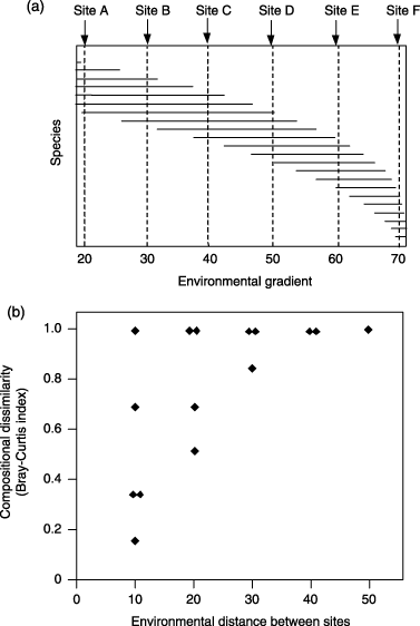
Hypothetical example illustrating the problems discussed in the text relating to the application of linear matrix regression to large-scaled ecological data sets. (a) Species’ distributions (horizontal lines) in relation to a hypothetical environmental gradient, with six survey sites positioned along this gradient. (b) Plot of compositional dissimilarity vs. environmental distance for all possible pairwise combinations of the six survey sites.
The second type of nonlinearity of interest here relates to the rate of compositional turnover along environmental gradients. Linear matrix regression assumes that this rate remains constant (or stationary) across the entire range of each environmental variable. Yet marked violations of this assumption are commonly encountered in real-world data sets (Whittaker, 1977; Wilson & Mohler, 1983; McNaughton, 1994; Oksanen & Tonteri, 1995; Simmons & Cowling, 1996). This is partly because environmental variables are measured on essentially arbitrary scales — e.g. log-transformed mean annual rainfall may provide better concordance with observed patterns in compositional turnover than untransformed rainfall. The example presented in Fig. 1 illustrates how variation in the rate of turnover along an environmental gradient can limit the ability of matrix regression to detect and model such a relationship. Site pairs A-B, B-C, C-D, D-E, and E-F all exhibit the same level of separation when measured against the depicted environmental gradient. However, because the rate of compositional turnover increases as one moves from left to right across this gradient, these equidistant site-pairs exhibit considerable variation in compositional dissimilarity (reflected in the vertical spread of points for environmental distance = 10 in Fig. 1b). As for the first type of nonlinearity, this second problem is likely to be more acute for extensive study areas spanning long environmental gradients.
Reformulating matrix regression as a generalized linear model
GDM is an extension of matrix regression designed specifically to accommodate both types of nonlinearity described above (Ferrier, 2002; Ferrier et al., 2002). The curvilinear relationship between ecological separation and compositional dissimilarity is addressed by reformulating the approach as a generalized linear model (McCullagh & Nelder, 1989). In keeping with other generalized linear models (e.g. logistic regression), this particular model is specified in terms of two functions: (1) a link function defining the relationship between the predicted response µ (in this case compositional dissimilarity between a pair of sites) and the so-called ‘linear predictor’η (in this case a scaled combination of intersite distances based on any number of environmental or geographical variables, as in the right-hand side of Equation 2); and (2) a variance function defining how the variance of µ depends on the predicted mean.
While different link functions may be appropriate for different measures of compositional dissimilarity (and therefore warrant further investigation), we have found the following link (presented here in inverse form) to have general utility in applications employing the Bray–Curtis index:
 (3)
(3)Given that the Bray–Curtis index is essentially a proportion (i.e. the number of species present at one site but not the other, expressed as a proportion of the sum of the total number of species, s, at each site), we employ the binomial variance function:
 (4)
(4)Other possible variance functions, including that based on the beta distribution (Ferrari & Cribari-Neto, 2004), deserve further consideration.
Also worthy of further consideration is the possibility of applying GDM to dissimilarities that have already been adjusted to compensate for the curvilinear relationship with ecological distance — e.g. by applying non-metric or hybrid multidimensional scaling (Faith et al., 1987) or by estimating extended dissimilarities (De’ath, 1999). In these situations the link function employed in GDM might be more appropriately defined as linear rather than curvilinear. However, more work is needed to determine whether such preprocessing of dissimilarities (through analysis of the biological data alone, without reference to the environmental data) confers any particular advantage over accommodating the curvilinear relationship, with ecological distance more directly within GDM (through combined analysis of the biological and environmental data).
Addressing non-stationarity in rates of compositional turnover
Extending this generalized linear version of matrix regression to address the second source of nonlinearity — that relating to variation in the rate of compositional turnover along environmental gradients — presents a more difficult challenge. Based on first impressions one may be tempted to approach this by simply converting the generalized linear model described above to a generalized additive model (Hastie & Tibshirani, 1990). This would involve replacing the linear terms comprising η with nonlinear functions fitted using, for example, scatterplot smoothing. However, because such an approach would transform pairwise distances derived from an environmental variable, not the variable itself, it would contribute little to solving the problem of interest here. This should be apparent from the example depicted in Fig. 1, in which site-pairs A-B, B-C, C-D, D-E, and E-F would all be assigned the same value in a matrix of pairwise environmental distances, and would therefore remain equivalent no matter how these distances were transformed.
GDM approaches this problem by fitting nonlinear functions directly to the environmental variables themselves, rather than to the pairwise distances derived from these variables. The general form of η in this approach is therefore:
 (5)
(5)The challenge now becomes one of fitting functions, fp(xp), to the environmental variables such that a model based on distances measured from these functions, fp(xpi) –fp(xpj), provides the best-possible fit between predicted and observed compositional dissimilarity. In GDM we make the reasonable assumption that compositional dissimilarity can only increase, not decrease, with increasing separation of sites along an environmental gradient. The functions, fp(xp), are therefore constrained to be monotonic. To ensure both monotonicity and flexibility of shape, each of these functions is fitted as a linear combination of I-spline basis functions (Ramsay, 1988):
 (6)
(6)where Ipk is the kth I-spline for variable xp and apk is the fitted coefficient for Ipk, subject to the constraint apk ≥ 0.
The I-spline basis functions are analogous to terms in a polynomial regression. However, because I-splines are themselves monotonic, any function derived by combining I-splines for a given environmental variable will also be monotonic, provided that all fitted coefficients are non-negative. Flexibility, or potential complexity, in the shape of the derived function for each variable is determined by the number of I-splines employed (mp in the above equation). A detailed description of I-splines, and their calculation, is beyond the scope of this paper. Further information is available in Ramsay (1988). Our use of I-splines in GDM was inspired largely by their prior application to a form of constrained multidimensional scaling by Winsberg & De Soete (1997).
Combining Equations 5 and 6 we can now reformulate η as:
 (7)
(7)or more simply:
 (8)
(8)This formulation is particularly convenient because it opens the way to fitting the required coefficients, apk, using the maximum-likelihood estimation approach commonly employed in other forms of generalized linear modelling (McCullagh & Nelder, 1989).
Model fitting
Fitting a GDM model to biological and environmental data from a set of survey sites involves the following steps:
- 1
Calculate compositional dissimilarity, d, between all possible pairs of survey sites (e.g. using the Bray–Curtis index).
- 2
For each environmental variable, xp, derive a set of mp I-spline basis functions and calculate the value of each survey site against each of these functions, Ipk(xp).
- 3
For each of the I-spline basis functions generated in Step 2, calculate the absolute difference in value between sites i and j, |Ipk(xpi) – Ipk(xpj)|, for all possible pairs of sites, and save these distances as ΔIpk.
- 4
If geographical distance between sites is required as an explanatory variable, then derive a set of I-spline basis functions directly from this distance. In other words, if gij is the geographical distance between sites i and j, then the relevant ΔIpk is now calculated simply as Ipk(gij). The same approach can be applied to other ‘distance variables’ enabling, for example, compositional dissimilarity in one biological group to be used as an explanatory variable for dissimilarity in another group (e.g. Steinitz et al., 2005).
- 5
Use maximum likelihood estimation to fit coefficients, apk, to the I-spline basis functions. This can be achieved using the iteratively re-weighted least squares (IRLS) algorithm (McCullagh & Nelder, 1989), with compositional dissimilarity as the response and the series of derived ΔIpk variables as predictors, and with link and variance functions as defined in Equations 3 and 4. The only non-standard requirement of this step is that all fitted coefficients must be non-negative to ensure monotonicity in fp(xp). This is readily achieved by replacing the least-squares regression normally employed within the IRLS algorithm with a non-negative least-squares regression.
Model selection and significance testing
The predictors included in a model, and the number of I-spline basis functions employed for each predictor (controlling the allowable complexity of the nonlinear transformation of that predictor), can be determined using various automated selection strategies, including forward-selection, backward-elimination, and stepwise procedures. As for linear matrix regression (Legendre et al., 1994), when these procedures are applied to GDM all significance testing must be performed using matrix permutation. The significance of adding or removing a predictor (or an I-spline basis function for any given predictor) is evaluated by first calculating the difference in deviance between two models — i.e. one with, and the other without, the predictor (or I-spline basis function) of interest. The deviance of each model is estimated as for any other form of generalized linear model (McCullagh & Nelder, 1989), employing the link and variance functions defined in Equations 3 and 4. This observed difference in deviance is then compared to a distribution of differences obtained by repeatedly fitting the two models using a large number of random permutations of the order of sites in the response (compositional dissimilarity) matrix.
A simple example
Figure 2 presents an example of a GDM model (Faith & Ferrier, 2002) fitted to rainforest-tree data from 34 plots in Panama (this data set is described by Condit et al., 2002). Several previous studies have analysed this same data set using a linear matrix regression (Duivenvoorden et al., 2002; Ruokolainen & Tuomisto, 2002; Chust et al., 2006). The model includes three predictors: precipitation, elevation, and geographical distance (two other environmental variables were considered in fitting the model, but were removed by a backward-elimination procedure). The nonlinear monotonic functions fitted for precipitation and geographical distance are derived from three I-spline basis functions, while that for elevation is derived from four I-splines. These fitted functions convey two important types of information. First, the maximum height reached by each function provides an indication of the total amount of compositional turnover (beta diversity) associated with the environmental gradient concerned, holding all other variables constant. Second, the slope of each function provides an indication of the rate of compositional turnover, and how this rate varies along the gradient concerned.
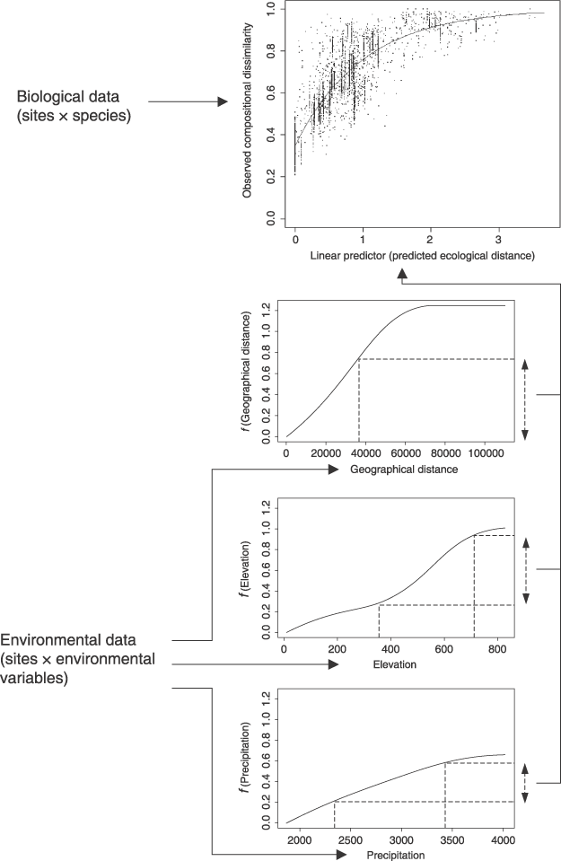
Example of a GDM model (Faith & Ferrier, 2002) fitted to Panamanian rainforest-tree data (this data set is described by Condit et al., 2002).
The plot of observed compositional dissimilarity (dij) vs. the linear predictor (ηij), indicates the fit between observed and predicted dissimilarity (the latter is represented by the curved line, which is the inverse-link function of the model). We refer to the linear-predictor axis of this plot as ‘predicted ecological distance’, to conform with the terminology employed by Gauch (1973) and Faith et al. (1987) in their descriptions of the curvilinear relationship between ecological distance and observed compositional dissimilarity.
EXTENSIONS
The basic GDM approach described above is very flexible, and can be extended to incorporate many different types of biological and environmental data. In this section we briefly outline some of these possibilities.
Incorporating nominal-scaled predictors
The mathematical description of GDM presented above assumes that environmental predictors are continuous variables or, at least, that these variables consist of ordered categories (e.g. classes of increasing soil fertility). However, some environmental variables of potential importance in modelling beta diversity may consist of disordered categories, including vegetation (or habitat) types or geological classes. At least three different approaches can be used to incorporate such variables into GDM: (1) Assign each pair of sites a distance of zero if they occur in the same class, or one if they occur in different classes, and then treat this binary distance measure in the same manner as geographical distance (see ‘Model fitting’ above). (2) Based on expert opinion, rate each possible pair of classes in terms of the perceived ecological difference between these classes (e.g. on a scale of 0–1), and then use these ratings as a more refined measure of distance between site pairs. (3) Use the ratings from the previous approach to perform a principal coordinate analysis (metric multidimensional scaling) of the classes, thereby generating a series of principal coordinate axes that can then be treated as continuous environmental variables in GDM.
Incorporating extended measures of geographical separation
Straight-line distance (or ‘map distance’) is just one of many possible approaches to measure geographical separation of sites. For example, if information on the relative impedance (or cost) to biological dispersal across different parts of a landscape is available as a spatial surface, then the separation of two sites can be measured as some function of the impedance accumulated along the least-cost path connecting these sites. In the example depicted in Fig. 3 the least-cost path between each pair of sites was derived by assuming that the impedance of any other grid-cell in the study area is proportional to the difference in elevation between that cell and the mean elevation of the two sites concerned. In other words, a GDM analysis employing this measure would treat high-elevation sites as being more isolated geographically if they are separated by low-elevation barriers, and vice versa. This approach could be readily extended to incorporate more sophisticated measures of biogeographical isolation based, for example, on palaeoclimatic reconstruction.
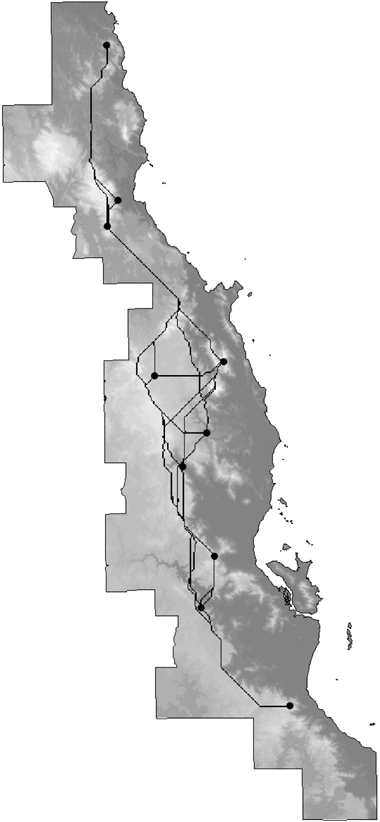
Least-cost paths generated between all pairs of 10 insect survey sites in the Australian Wet Tropics. These sites are a subset of a much larger set of insect sites. The shading depicts elevation (higher elevation areas are lighter), which was the variable used to estimate impedance to movement (see text for details). (The insect survey sites were kindly provided by Geoff Monteith, Queensland Museum.)
Incorporating phylogenetic/taxonomic information
Measures of compositional dissimilarity employed in community ecology rarely incorporate any information on phylogenetic relationships between the species involved (Webb et al., 2002). Yet such information may help to shed more light on patterns of beta diversity, particularly if these patterns are being viewed from an evolutionary, as opposed to strictly ecological, perspective. As part of our work on GDM we have therefore developed a new method for extending traditional measures of compositional dissimilarity to incorporate information on phylogenetic relationships.
Using the Bray–Curtis measure as an example, recall from Equation 1 that this index is calculated as a function of A, the number of species shared by two sites, and B and C, the numbers of species occurring at one site but not the other. Now assume that a phylogenetic tree is available for the group of species of interest. By adopting principles of the phylogenetic diversity (PD) approach of Faith (1992), we can factor phylogeny into the Bray–Curtis measure by simply redefining A, B, and C in terms of the total phylogenetic branch length shared by the two sites vs. the remaining total branch length unique to one site or the other (see Fig. 4). This same technique can be applied to any of the extensive family of dissimilarity measures based on the quantities A, B, and C (Koleff et al., 2003), e.g. the Jaccard index. In the absence of an appropriate phylogeny, our approach can instead be applied to a tree representing the hierarchical taxonomic relationships between species (genus, family, order, etc.).
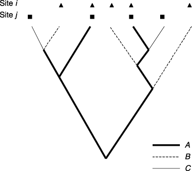
Hypothetical phylogeny for species occurring at two sites, i and j. This phylogenetic information can be used to derive an extended version of the Bray–Curtis dissimilarity index by redefining the quantities A, B, and C (from Equation 1) in terms of phylogenetic branch length, where A is the total branch-ength shared by the two sites, B is the total branch length unique to site i, and C is the total branch length unique to site j.
Incorporating presence-only biological data
To this point our description of GDM has assumed that the biological data used to fit a model have been collected through consistent application of a given survey technique at all sites. In this situation, each species in the group of interest has been recorded as either present or absent at each and every survey site in the data set. However, much of the world's data on biodiversity is not in this form. Data derived from the extensive biological collections of museums and herbaria contain extremely valuable information on locations where species have been recorded as present (i.e. collected) but offer virtually no information on the other locations that were searched unsuccessfully for these species (Graham et al., 2004).
GDM has, in a few cases, been applied to such data sets by using the combined set of locations from which one or more species within the group of interest have been collected, as an approximate indicator of locations searched for each species within the group (Ferrier et al., 2004; Elith et al., 2006). In other words, if a species has not been collected at one of these locations then it is assumed to be absent for the purposes of the GDM analysis. Differences in collection effort between locations are then addressed to some extent by the weighting for number of species recorded at each site in the GDM variance function (Equation 4). This ensures that pairs of sites with few species recorded carry less weight, and therefore have less influence, in the fitting of a model than site-pairs with larger numbers of species. These approaches to applying GDM to biological collection (presence-only) data sets should, however, be regarded as approximate only, and require further evaluation and refinement.
APPLICATIONS
Once a GDM model has been fitted to available biological data for a study area, this model can be used to predict the compositional dissimilarity expected between any two locations, knowing only the position of these locations in relation to each of the environmental and geographical predictors employed in the model. If all of these predictors are available as spatial surfaces within a geographical information system (GIS) then this opens the way to extrapolating patterns of compositional turnover (beta diversity) across an entire study area. Such extrapolation can, in turn, provide the basis for a wide range of biodiversity assessment and planning activities, some of which we outline below (see also Fig. 5).
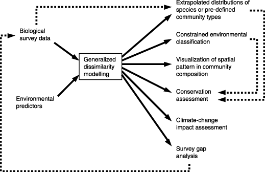
Applications of generalized dissimilarity modelling.
Visualizing spatial pattern in community composition
By applying multidimensional scaling (metric or non-metric) to predicted compositional dissimilarities between pairs of locations (grid cells) within a region, these locations can then be mapped against the resulting ordination axes. Assigning the first three ordination axes to the red, green, and blue (RGB) bands of a colour image provides an effective means of visualizing spatial pattern in community composition (Fig. 6a). Grid cells mapped in a similar colour are predicted to have similar biological composition, while cells mapped in a very different colour are predicted to be highly dissimilar in composition.
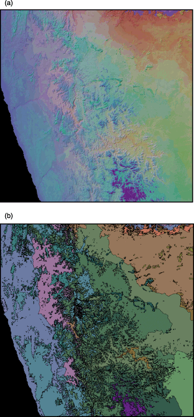
(a) A visualization of spatial pattern in plant community composition in the Namaqualand region of South Africa, derived by applying metric multidimensional scaling to compositional dissimilarities predicted by a GDM model fitted to floristic survey data. Areas of similar colour are predicted to be floristically similar. (b) A 20-class classification of the region derived from the same predicted dissimilarities. (All floristic and environmental data were kindly provided by Philip Desmet, University of Cape Town.)
In a region containing a very large number of grid cells it will usually not be feasible to apply multidimensional scaling directly to all possible pairs of cells. In this situation the scaling can be performed using a randomly selected sample of cells. Ordination scores for the other cells are then assigned through some form of interpolation, such as that based on k-nearest neighbours, using weights proportional to the predicted similarity (the complement of predicted dissimilarity) between sampled and unsampled cells. A similar approach to visualizing spatial pattern in beta diversity has been described recently by Thessler et al. (2005).
Constrained environmental classification
Predicted compositional dissimilarities can also be used as a basis for clustering grid cells into discrete classes, employing some form of numerical classification (Fig. 6b). As for the multidimensional scaling approach described above, the initial classification may need to be performed for a random sample of cells, with each of the other cells then assigned to one of the resulting classes based on a k-nearest neighbour analysis. Classes mapped using this approach can be employed in conservation assessment and planning in the same manner as classes derived through other forms of environmental domain (or cluster) analysis (Mackey et al., 1989; Fairbanks & Benn, 2000; Hargrove & Hoffman, 2004; Trakhtenbrot & Kadmon, 2005). However, unlike these other approaches that classify a region based on environmental similarity (or dissimilarity) alone, the classification approach described here is based on predicted biological dissimilarity. This is therefore a form of constrained environmental classification, in which available biological data have been used to inform the transformation and weighting of environmental variables such that classes derived from these variables will match real biological patterns as closely as possible.
Extrapolating distributions of species or predefined community types
The transformation of multidimensional environmental space (and, optionally, geographical space) performed by GDM may also serve as a useful pre-processing step in modelling the distributions of individual species. As part of a recent comparative study of the performance of various species-modelling techniques (Elith et al., 2006), we linked GDM to a simple kernel regression procedure (Lowe, 1995), thereby modelling the density of presence records for each species within a GDM-transformed environmental space (Fig. 7). The predictive performance of this approach compared very favourably with other better-known techniques for modelling species distributions. We have used a similar approach to model distributions of vegetation communities in a number of recent vegetation mapping projects within New South Wales, Australia (e.g. Department of Environment and Conservation, 2004). In this case, records for individual species are replaced by records for each of a set of community types derived, for example, from a separate numerical classification of floristic plots.
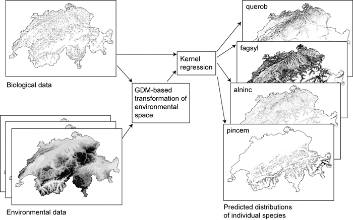
Tree-species distributions in Switzerland modelled by linking GDM to a simple kernel regression procedure, thereby modelling the density of presence records for each species within a GDM-transformed environmental space. See Elith et al. (2006) for further detail. Key: alnic = Alnus incana, fagsyl = Fagus sylvatica, pincem = Pinus cembra, querob = Quercus robur. The data used in this example were generated for a working group at the National Center for Ecological Analysis and Synthesis (NCEAS), Santa Barbara, USA, led by Town Peterson and Craig Moritz. The data were kindly provided by Antoine Guisan (University of Lausanne) and Nicolas Zimmerman (WSL Switzerland).
Survey gap analysis
The ability to predict patterns of compositional turnover in unsurveyed parts of a region provides an ideal basis for directing new survey or collection effort to locations that best complement those already surveyed, thereby maximizing the likelihood of encountering species not yet sampled within the region. We have now applied this approach in a number of regions by linking GDM to a survey-gap analysis procedure (Ferrier, 2002; Funk et al., 2005; Fig. 8) based on the environmental diversity (ED) technique of Faith & Walker (1996). As described by Ferrier (2002) this approach offers a solid foundation for incremental refinement of biological information in data-poor regions. Predictions from an initial GDM model, based on best-available biological data, can be used to locate additional survey sites. Data from these new sites can, in turn, be used to refine the model of compositional turnover, thereby providing an improved basis for selecting any further sites.
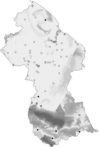
Application of GDM to a survey-gap analysis of termite collection sites in Guyana. The open circles depict existing collection sites, to which the GDM model was fitted. The closed circles depict six proposed survey locations selected by the analysis as best complementing the existing sites. The various shades of grey indicate the relative priority of remaining areas for further survey. (The termite data were kindly provided by the Program for the Biological Diversity of the Guianas at the Smithsonian Institution.)
Conservation assessment
In the most extensive application of the technique to date, GDM played a major role in an assessment of the representativeness of the world's protected area system associated with the 5th World Parks Congress in 2003 (Ferrier et al., 2004). Modelled patterns of compositional turnover within all of the planet's terrestrial biomes, combined with information on broad patterns of species richness, were used to estimate the proportion of species-level biodiversity represented in protected areas, with a particular emphasis on plants and invertebrates. This assessment of representativeness was performed using a novel analytical technique combining elements of ED analysis with principles of the species-area relationship (see Ferrier et al., 2004 for details). This same technique has been used more recently to assess expected levels of biodiversity loss in Madagascar resulting from past habitat lost (T. Allnutt, pers. comm.).
Climate-change impact assessment
The GDM-based approach to conservation assessment developed by Ferrier et al. (2004) also has potential applicability to predicting climate-change impacts. To date, most predictions of distributional shifts expected to result from climate change have been based either on modelling of individual species or on modelling of discrete biomes or community types (Ferrier & Guisan, 2006). As illustrated by the example depicted in Fig. 9, GDM offers an alternative approach in which distributional shifts can be assessed in relation to continuous gradients of compositional turnover. This approach may allow potential climate-change impacts to be assessed more rapidly, at a relatively fine resolution, across extensive regions of the planet with sparse biological data. Unlike other community-level approaches to predict distributional shifts in response to climate change, this approach does not assume that species will move together as fixed community types. The approach may therefore be relatively robust to high individuality in species’ responses, provided that emergent rates of spatial turnover in community composition along environmental gradients remain reasonably constant in the face of climate change.
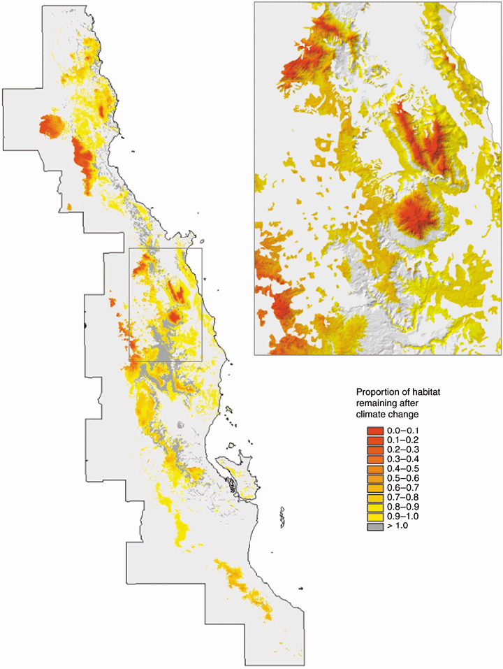
A trial application of GDM to climate-change impact assessment in the Australian Wet Tropics. The assessment is based on a GDM model fitted to rainforest plant data. The proportional change in habitat area following climate change is estimated for each rainforest grid-cell in the region, using an adapted version of the GDM-based technique proposed by Ferrier et al. (2004) for assessing biological representativeness. The future climate layers were kindly provided by Susan Cameron (University of California, Davis) and were derived by downscaling the difference between current and future climate for the CCM3 2xCO2 scenario generated by Govindasamy et al. (2003), and adding this difference to current fine-scaled climate surfaces (Rainforest CRC, 2003). (The plant data used to fit the GDM model were kindly provided by Andrew Ford, CSIRO Sustainable Ecosystems.)
FUTURE DIRECTIONS
GDM provides a powerful means of analysing and predicting spatial patterns in compositional turnover (beta diversity) across very large regions. The approach can help make more effective use of best-available biological and environmental data in a wide range of assessment and planning activities. However, the method is still relatively new and more work is needed to refine and extend various aspects including, for example, techniques for estimating confidence intervals around predicted compositional dissimilarities and for better accommodating interactions between environmental predictors. More attention also needs to be directed to evaluating the predictive performance of GDM in different environments and under different conditions, and comparing the performance of GDM with other species-level and community-level modelling strategies.
ACKNOWLEDGEMENTS
Our thinking on GDM has benefited greatly from discussion and interaction with Dan Faith, Jake Overton, Jim Thompson, and Hanna Tuomisto. We thank sincerely all those individuals and institutions who so generously provided data for the examples included in this paper: Susan Cameron (University of California, Davis), Philip Desmet (University of Cape Town), Antoine Guisan (University of Lausanne), Andrew Ford (CSIRO Sustainable Ecosystems), Geoff Monteith (Queensland Museum), the Program for the Biological Diversity of the Guianas (Smithsonian Institution), and Nicolas Zimmerman (WSL Switzerland). We also thank the Universidad Internacional de Andalucía, sede Antonio Machado, Baeza, Spain, for organizing the workshop ‘Predictive modelling of species distributions, new tools for the XXI century’. Finally we thank Town Peterson and an anonymous reviewer for helpful comments on the manuscript.


