Pareto-Improving Water Management over Space and Time: The Honolulu Case
Abstract
We model welfare gains from efficient allocation of groundwater over space and time relative to the status quo policy of financial cost recovery. In order to promote political feasibility, an intertemporal compensation plan is devised that renders the reform Pareto-improving. Gainers from the reform finance the compensation in proportion to their benefits through a block-pricing scheme. For the Honolulu case, only 7% of the $441 million in gains to winners is needed to compensate losers from the reform. Future winners from the reform also repay the deficit created by the compensation package, much as state and local governments finance capital improvements.
Despite a voluminous literature on groundwater management (Koundouri 2004 for a survey), proposals to induce efficient use through pricing or quantity regulations have often been politically infeasible (Postel 1999, p. 235–36; Dinar 2000; Johansson 2000). A common problem with these proposals is that current water consumers are called on to sacrifice in order that future users will be better off (Feinerman and Knapp 1983). When gains from efficiency pricing are far in the future and are realized after initial losses (e.g., from paying higher prices), then present users may or may not accept the switch to efficiency pricing, even if the present value of the future gains is more than the present value of the initial losses. Present users may not be sufficiently long lived to enjoy the future gains or sufficiently interested in the welfare of future generations, or just may not have enough foresight and confidence to expect the future gains. Present users are politically more influential than future users (some of whom are unborn) and are therefore able to block reforms (Olson 1965; Dinar and Wolf 1997).
To avoid the problems of political infeasibility arising from a policy's differential impact, a mechanism can be provided for compensating those who lose welfare due to efficient management. Compensation possibilities to enhance political feasibility have been discussed in general (Krueger 1992; Williamson 1994) but have not been explicitly developed in a spatial-temporal framework. In this article, we use the urban Honolulu water district to examine how welfare impacts of efficiency pricing vary over water users at different locations and times, and provide a mechanism to compensate those users who lose welfare due to the switch to efficiency pricing, by transferring some gains from welfare-gaining users. Our objectives are to: (a) compute the efficient allocation of water across time and across locations, (b) compute efficiency prices needed at the margin to support the efficient allocation as a decentralized equilibrium, (c) simulate the effects of the status quo policy of pricing water at average cost of extraction and distribution, (d) estimate the topographic and temporal distribution of welfare gain/loss to users by switching from the status quo to efficiency pricing, and (e) define a lump-sum compensation scheme such that the switch to efficiency pricing causes no user to be a net loser.
The rest of the article is organized as follows: The next section provides a theoretical apparatus for modeling the status quo and efficient management scenarios, calculating the welfare effects of switching from one to the other, and constructing a compensation mechanism. In the application section, we determine efficiency prices and estimate the welfare effects of switching from status quo to efficiency pricing in the Honolulu case. In the compensation section, we provide a method for compensating those who lose welfare as a result of switching from status quo to efficiency pricing and a mechanism to finance the compensation, and discuss related equity issues. The final section summarizes the major findings and discusses possible extensions.
The Model
Groundwater aquifers that provide freshwater in coastal areas, such as Honolulu, usually exhibit Ghyben-Herzberg lens geometry (Mink 1980), in which a freshwater layer floats on a saltwater layer that percolates from the ocean. A higher freshwater head level increases water pressure within the aquifer and increases leakage from the aquifer toward the ocean, causing net recharge to vary inversely with head. If the freshwater is extracted faster than the net recharge, the freshwater head falls and the saltwater rises. The rising saltwater can ultimately reach the bottom of the current well systems that will then begin to pump out saltwater. The freshwater head, therefore, needs to be constrained from falling below the level at which the wells would begin to turn saline. If more freshwater is required than that allowable under the constraint, it must be obtained through desalination of seawater, which serves as a backstop.
Users in Honolulu are distributed over different elevations with different distribution costs (table 1) and water demand is growing with increasing population and per capita income. The status quo policy of the city-owned water utility, Honolulu Board of Water Supply (HBWS) is to price water equal to the marginal physical cost of providing water, ignoring the user cost. Further inefficiency is introduced as the water utility sets a uniform price for users at all elevations, in effect cross-subsidizing high-elevation users. Efficient use would require correcting the spatial inefficiency as well as intertemporal optimization. Construction of a compensation scheme requires explicit disaggregation of consumers over space and time, and analysis of the distributional consequences of efficient management versus the existing, inefficient management practice.
To adequately represent the local conditions, we require an operational model of an exhaustible groundwater aquifer with variable recharge, the possibility of well-salinization, desalting as a backstop source of freshwater, and a growing demand for water. The model must allow us to derive water usage under temporally and spatially optimal policy as well as under the status quo policy, and estimate welfare distribution under both policies. The required model is obtained by combining the temporal optimization approach (e.g., Burt 1967, 1970; Brown and Deacon 1972; Gisser and Sanchez 1980; Feinerman and Knapp 1983; Krulce, Roumasset, and Wilson 1997) and the spatial optimization approach (e.g., Tolley and Hastings 1960; Chakravorty and Roumasset 1991; Chakravorty, Hochman, and Zilberman 1995) into a single analytical framework.1 The model is adapted to solve for water allocation under status quo as well as optimal management.
| Elevation Category (i) | Average Elevation (Feet) | Constant of the Demand Function: Ai(mgd) | Distribution Cost: cdi($/Thousand Gallons) | Current Status Quo Price: psq($/Thousand Gallons) | Effective Price: (psq − cdi) ($/Thousand Gallons) |
|---|---|---|---|---|---|
| 1 | 0.00 | 67.58 | 1.74 | 1.97 | 0.23 |
| 2 | 447.89 | 13.40 | 2.09 | 1.97 | −0.12 |
| 3 | 819.47 | 1.83 | 2.51 | 1.97 | −0.54 |
| 4 | 1,071.08 | 0.64 | 3.22 | 1.97 | −1.25 |
| 5 | 1,162.57 | 0.13 | 4.14 | 1.97 | −2.17 |
| 6 | 1,344.00 | 0.09 | 5.28 | 1.97 | −3.31 |
- a Source: Honolulu Board of Water Supply (2002).
Water is extracted from a coastal groundwater aquifer that is recharged from a watershed and leaks into the ocean from its ocean boundary depending on the aquifer head level, h, (measured as the vertical distance between sea level and the top of the freshwater layer). Net recharge (recharge minus leakage), w, is a positive, decreasing, concave function of head, that is, w(h) ≥ 0, w′ (h) < 0, w″ ≤ 0. The aquifer head level, ht, changes over time according to: 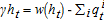 , where qit is the quantity extracted for consumption at elevation i at time t, and γ is the factor of conversion from volume of water in gallons (on the R.H.S.) to head level in feet. The minimum head level required to avoid salt concentrations exceeding the EPA limit is hmin.
The unit cost of the backstop is cb. The unit cost of extraction is a function of the vertical distance water has to be lifted, f = e − h, where e is the elevation of the well location. At lower head levels, it is more expensive to extract water because the water must be lifted over a longer distance, f. The extraction cost is, therefore, a positive, increasing, convex function of the lift, c(f) ≥ 0, c′(f) > 0, c″(f) ≥ 0. Since the well location is fixed, we can redefine the unit extraction cost as a function of the head level: cq(h) ≥ 0, where c′q(h) < 0, c′′q(h) ≥ 0. The total cost of extracting water from the aquifer at the rate q given head level h is cq(h)q. The cost of transporting a unit of water to users in category, i, is cid.
Users are distributed over different elevation categories. The consumption of groundwater in elevation category i at time t is qti and the consumption of the backstop is bit⋅Di(pit, t)(= qit + bit), is the water demand at price pit at time t.
We first model water allocation under status quo management and then under efficient management. The differences in welfare distribution under the two regimes are then examined and used to derive a mechanism to compensate those who lose welfare when the efficient allocation is implemented.
Status Quo Management
In the status quo scenario, price is set at the marginal cost of extraction and distribution, averaged over all users. Extraction is equal to the quantity demanded at the status quo price, until the groundwater head has reached its minimum, after which extraction is limited to recharge, and additional water is obtained through desalination. Once desalination is needed, water price under the status quo system is set equal to a weighted average of extraction and desalination costs.
 (1)
(1) , and htsq is the head level at time t under the status quo scenario and changes as
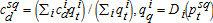
  , where
  is the quantity extracted at time t. After the head level reaches the minimum allowable point, hmin, the rate of groundwater extraction is held constant at w(hmin) and any excess demand is met from the desalination backstop. The status quo (average cost) price, psqt, is, therefore, a volume-weighted average cost of water from the two sources (desalination and underground aquifer).
Efficient Management
A hypothetical social planner chooses the extraction and backstop quantities over time to maximize the present value (discounted at rate, r) of net social surplus, and corresponding efficiency price paths are computed for each user category over time.
 (2)
(2)
 (3)
(3) (4)
(4) (5)
(5) (6)
(6) (7)
(7) (8)
(8) . Combining this expression with equations (4), (5), and (8) and rearranging, the following arbitrage condition is obtained:
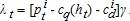
 (9)
(9)Equation (9) implies that at the margin, the benefit of extracting water must equal the actual costs for extraction and distribution plus the marginal user cost associated with both higher future extraction costs and the forgone use of the marginal unit when its demand price is higher. Thus, if water is priced at physical costs alone, as is common in many areas, marginal user cost is ignored and overuse will occur. Equation (9) also implies that the price in two elevation categories should differ only by the difference between their distribution costs.2
 to the L.H.S., we get the following equation of motion
 (10)
(10) (11)
(11)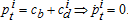 . We can substitute pit = cb + cid into (9) to get
 (12)
(12)If the head-level constraint is nonbinding at steady-state, αt = 0, and (12) can be solved for the steady-state head level. If the constraint is binding, the steady-state head level is hmin. We denote the steady-state head level as hfin. At hfin, the quantity extracted from the aquifer must equal the net recharge to the aquifer. With exogenously growing demand, the quantity consumed would continue to increase. The excess of quantity demanded over net recharge is supplied by desalination.
Revenue
 (13)
(13) (14)
(14) (15)
(15)The switch from status quo to efficiency pricing changes the welfare of the users in category i at time t by zit = vit − yit, which may be positive or negative. If zit > 0 for a consumer, he/she is a gainer and if zit < 0, he/she is a loser.
Application
We apply the model to the freshwater market supplied from the Honolulu groundwater aquifer. We calibrate the above model and solve for efficiency prices, and estimate welfare effects of switching to efficiency pricing.
Calibration
The volume of water stored in the Honolulu aquifer4 depends on the head level, the aquifer boundaries, the Ghyben-Herzberg lens geometry, and rock porosity. Although the freshwater lens is a paraboloid, the upper and lower surfaces of the aquifers are nearly flat (see Mink 1980). Thus, volume of aquifer storage is modeled as linearly related to the head level. Using GIS aquifer dimensions (Office of Planning 2004) and effective rock porosity of 10% (following Mink), the Honolulu aquifer has 61 billion gallons (bg) of water stored per foot of head. This value is used to calculate the conversion factor from head level in feet to volume in billion gallons. Extracting 1 bg of water from the aquifer would lower the head by 1/61 or 0.0163934 feet, giving us γ = 0.0163934 ft/bg. Econometric estimate of net recharge, w, as a function of the head level, h, is w(h(t)) = 157 − 0.24972h(t)2 − 0.022023h(t), where l is measured in million gallons per day (mgd).
We calculate the minimum allowable head level to be 15 feet. The deepest wells in the Honolulu aquifer are at Beretania pumping station and have a bottom depth of about 600 feet. This well system will be the first to go saline as the freshwater head level will fall and the saltwater interface will rise to meet the well bottom (thereby making it saline). The current head level at this location is about 22 feet. Using a 1:40 ratio of freshwater head to depth of saltwater interface in a Ghyben-Herzberg freshwater lens (as calculated by Mink), we get current depth of the interface at 880 feet below sea level. When this interface rises to the bottom of the Beretania wells (600 below sea level), the wells will turn saline. Using the 1:40 ratio, this implies a freshwater head level of 15 feet.
The cost is a function of elevation (and, therefore, the head level), specified as 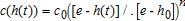 , where c0 is the initial extraction cost when the head-level h(t) is at the current level, h0 = 22 feet (at Beretania wells). There are many wells from which the freshwater is extracted and, using a volume-weighted average cost, the initial average extraction cost in Honolulu is $0.16 per thousand gallon (tg) of water. Here, e is the average elevation of these wells and is estimated at 50 feet, and n is an adjustable parameter that controls the rate of cost growth as head falls. We initially assume n = 2 and conduct sensitivity analyses for linear (n = 1) and highly convex (n = 3) cases. Since the head level does not change much relative to the elevation, the value of n does not affect the results appreciably. We calculate the distribution cost, cid, for each elevation category from pumping data (table 1). The unit cost (cb) of desalting in Honolulu is currently estimated at $7/tg. This includes the cost of desalting and an additional cost of transporting the desalted water from the desalination plant to the existing freshwater distribution network. Technical progress may lead to a lower desalination cost over time.5 We abstract away from explicitly modeling technical progress and provide sensitivity analyses for cb = $5, 6, and 8 (table 3).

| Parameter Values | Gain ($) | Loss ($) | Loss/Gain (%) |
|---|---|---|---|
| g = 1, r = 3, η = −0.25, cb = 7, n = 2 | 4.41492 × 10⁸ | 3.41286 × 10⁷ | 7.7303 |
| g = 2, r = 3, η = −0.25, cb = 7, n = 2 | 2.87016 × 10⁹ | 7.10178 × 10⁷ | 2.47435 |
| g = 3, r = 3, η = −0.25, cb = 7, n = 2 | 8.90351 × 10⁹ | 1.03764 × 10⁸ | 1.16543 |
| r = 1, η = −0.25, cb = 7, n = 2, g = 1 | 4.10026 × 10⁹ | 8.96464 × 10⁷ | 2.18636 |
| r = 2, η = −0.25, cb = 7, n = 2, g = 1 | 1.29086 × 10⁹ | 5.31298 × 10⁷ | 4.11585 |
| r = 3, η = −0.25, cb = 7, n = 2, g = 1 | 4.41492 × 10⁸ | 3.41286 × 10⁷ | 7.7303 |
| r = 4, η = −0.25, cb = 7, n = 2, g = 1 | 1.66164 × 10⁸ | 2.36151 × 10⁷ | 14.2119 |
| n = 1, g = 1, r = 3, η = −0.25, cb = 7 | 4.46321 × 10⁸ | 3.36008 × 10⁷ | 7.52839 |
| n = 2, g = 1, r = 3, η = −0.25, cb = 7 | 4.41492 × 10⁸ | 3.41286 × 10⁷ | 7.7303 |
| n = 3, g = 1, r = 3, η = −0.25, cb = 7 | 4.37378 × 10⁸ | 3.24464 × 10⁷ | 7.41839 |
| η = −0.15, cb = 7, n = 2, g = 1, r = 3 | 7.47648 × 10⁸ | 3.89001 × 10⁷ | 5.20299 |
| η = −0.25, cb = 7, n = 2, g = 1, r = 3 | 4.41492 × 10⁸ | 3.41286 × 10⁷ | 7.7303 |
| η = −0.3, cb = 7, n = 2, g = 1, r = 3 | 3.47041 × 10⁸ | 3.23112 × 10⁷ | 9.31051 |
| cb = 5, η = −0.3, n = 2, g = 1, r = 3 | 3.16384 × 10⁸ | 3.30352 × 10⁷ | 10.4415 |
| cb = 6, η = −0.3, n = 2, g = 1, r = 3 | 4.10837 × 10⁸ | 3.37025 × 10⁷ | 8.20340 |
| cb = 7, η = −0.25, n = 2, g = 1, r = 3 | 4.41492 × 10⁸ | 3.41286 × 10⁷ | 7.7303 |
| cb = 8, η = −0.3, n = 2, g = 1, r = 3 | 5.73062 × 10⁸ | 3.44064 × 10⁷ | 6.00397 |

Solution Algorithm
A computer algorithm is used to simultaneously solve the two differential equations, (4) and (10), using the initial (current) head level and the final (backstop) price as two boundary conditions. This yields optimal head level and price as functions of time (p*(t), h*(t)). We solve equation (12) to obtain the head level (hfin) in the final period (tfin). The value of tfin is then obtained by setting h*(tfin) = hfin. Welfare in each elevation category is computed as the area under that category's demand curve minus extraction and distribution costs (as in equation 3).
Results
Now we examine the time-paths of prices, head levels, and welfare, under the status quo and efficiency pricing scenarios.
Status Quo Management
The status quo price (figure 1a) starts at $1.97/tg and increases slightly over time due to the head level (figure 1b) drawdown through extraction and the resulting increase in extraction costs. Consumption (corresponding to the status quo price) in each elevation category is given in figure 1(c), and at selected intervals, in table 2, panel (a).
Higher-elevation users have larger per capita consumption. They are generally considered high-income consumers. Over time, consumption increases and the head level decreases until it reaches 15 feet, the minimum allowable7 to avoid aquifer salinity, in year 57. At this point, extraction must be adjusted such that head level does not fall further, that is, extraction must not exceed recharge. Thus, in year 57, consumption is partly supplied from the backstop source (desalination) and partly from the groundwater source. The price is therefore a volume-weighted average of the cost of the backstop and the cost of the groundwater. This results in a jump in the status quo price from $2.05 in year 56 to $2.86 in year 57. As a result, consumption falls in year 57. Afterward, as consumption continues to grow, more and more of it is supplied from the backstop source and the price (as a volume-weighted average cost) continues to increase toward the backstop price.

Status quo versus efficiency pricing: Prices, head levels, and quantities
| Year | Categ. 1 | Categ. 2 | Categ. 3 | Categ. 4 | Categ. 5 | Categ. 6 |
|---|---|---|---|---|---|---|
| (a) Consumption Under Status Quo (Gallons per Capita per Day) | ||||||
| 0 | 111 | 115 | 120 | 127 | 135 | 143 |
| 56 | 172 | 179 | 186 | 197 | 209 | 222 |
| 57 | 160 | 166 | 173 | 183 | 194 | 206 |
| 100 | 201 | 209 | 218 | 231 | 245 | 260 |
| (b) Efficiency Price ($/Thousand Gallons) | ||||||
|---|---|---|---|---|---|---|
| 0 | 1.98 | 2.33 | 2.75 | 3.46 | 4.38 | 5.52 |
| 76 | 8.74 | 9.09 | 9.51 | 10.22 | 11.14 | 12.28 |
| 100 | 8.74 | 9.09 | 9.51 | 10.22 | 11.14 | 12.28 |
| (c) Consumption Under Efficiency Price (Gallons per Capita per Day) | ||||||
|---|---|---|---|---|---|---|
| 0 | 111 | 111 | 112 | 112 | 113 | 113 |
| 48 | 141 | 143 | 146 | 148 | 151 | 153 |
| 68 | 138 | 142 | 146 | 151 | 156 | 161 |
| 76 | 140 | 145 | 149 | 155 | 161 | 167 |
| 100 | 171 | 175 | 181 | 188 | 195 | 202 |
| (d) Present Value of Revenue (Million $ per Annum) | ||||||
|---|---|---|---|---|---|---|
| 0 | 1.8 | 0.35 | 0.048 | 0.017 | 0.003 | 0.002 |
| 76 | 207.23 | 42.06 | 5.91 | 2.15 | 0.46 | 0.34 |
| 100 | 263.45 | 53.46 | 7.52 | 2.73 | 0.59 | 0.43 |
| (e) Size of the Free Block (Gallons per Capita per Day) for Revenue Return | ||||||
|---|---|---|---|---|---|---|
| 0 | 4.8 | 4.1 | 3.4 | 2.7 | 2.2 | 1.7 |
| 76 | 108.8 | 107.9 | 106.2 | 102.8 | 97.9 | 91.8 |
| 100 | 113.2 | 112.8 | 111.8 | 109.2 | 105.1 | 99.6 |
| (f) Present Value of Welfare Gain by Switching from Status Quo to Efficiency Pricing ($ per Day) | ||||||
|---|---|---|---|---|---|---|
| 0 | 450.775 | −358.065 | −119.355 | −80.665 | −26.645 | −26.645 |
| 56 | −1268.01 | −367.92 | −69.35 | −35.405 | −10.22 | −9.49 |
| 57 | 3639.05 | 642.4 | 75.19 | 18.615 | 2.19 | −0.365 |
| 76 | 3196.67 | 612.47 | 80.3 | 25.915 | 4.745 | 2.555 |
| 100 | 4054.785 | 804.825 | 110.23 | 38.325 | 8.03 | 5.11 |
| (g) Present Value of Per Capita Welfare Gain by Switching from Status Quo to Efficiency Pricing ($ per Capita per Day) | ||||||
|---|---|---|---|---|---|---|
| 0 | 0.002 | −0.009 | −0.02 | −0.04 | −0.07 | −0.102 |
| 56 | −0.006 | −0.008 | −0.012 | −0.017 | −0.024 | −0.03 |
| 57 | 0.017 | 0.015 | 0.013 | 0.009 | 0.004 | −0.001 |
| 76 | 0.014 | 0.014 | 0.013 | 0.012 | 0.010 | 0.008 |
| 100 | 0.0177 | 0.0178 | 0.0179 | 0.0178 | 0.0175 | 0.0168 |
| (h) Size of the Free Block (g/d/Capita) for Compensation and Revenue Return | ||||||
|---|---|---|---|---|---|---|
| 0 | 4.48 | 8.27 | 12.09 | 16.04 | 18.76 | 20.34 |
| 56 | 88.47 | 87.18 | 85.41 | 82.24 | 78.23 | 73.66 |
| 57 | 80.94 | 77.12 | 72.8 | 66.26 | 59.16 | 55.85 |
| 76 | 106.78 | 105.61 | 103.75 | 100 | 94.81 | 88.52 |
| 100 | 110.11 | 109.57 | 108.36 | 105.53 | 101.17 | 95.57 |
Efficient Management
The efficiency price (figure 1a) starts at $1.98/tg for the first elevation category and increases over time, faster than the status quo price, due to the head level (figure 1b) drawdown through extraction and the resulting increase in marginal user cost and extraction costs. Table 2, panel (b) gives prices for all elevation categories at selected intervals.
Higher elevations have higher prices due to larger distribution costs. The efficiency price in the lowest elevation category starts at $1.98/tg, which is very close to the status quo price of $1.97/tg, even though the former includes marginal user cost. This is because, under efficiency pricing, low-elevation users pay a lower distribution cost and do not have to subsidize distribution costs for higher elevations. Consumption (corresponding to the efficiency price) in each elevation category is given in figure 1(c), and at selected intervals, in Table 2, panel (c).
The head level decreases over time until it reaches the minimum allowable to avoid aquifer salinity, in year 76. After this point, extraction must be such that head level does not fall further, that is, extraction must not exceed recharge. Therefore, in year 76, consumption is partly supplied from the backstop source (desalination) and partly from the groundwater source.8 The efficiency price, thus, reaches the backstop price (plus distribution cost) and remains there.
The present value of revenue per capita is shown in figure 2(a), and total annual revenue, at selected intervals, is given in table 2, panel (d). The revenue is initially small as the efficiency price is only slightly higher than the status quo price (average cost). It is relatively large in the lowest elevation category, however, because of lower distribution costs. Over time, the efficiency price rises and the revenue generated increases.
To return this revenue, we use block-pricing where an initial block of a certain size is provided to the users free of charge. The size of the free block is adjusted as the amount of revenue collected changes over time as shown in figure 2(b), and at selected intervals, in table 2, panel (e). The size of the free block is smaller for higher-elevation categories because their distribution cost is larger and it costs more to provide them the free block. The size of the block increases over time as the revenue collected increases and is rebated via the free block.

Revenue, welfare change, free blocks, and financing of compensation under efficiency pricing
Switching from the status quo pricing to the above efficiency price system provides welfare gains, as shown at selected intervals, in table 2, panel (f). Per capita welfare gains by switching from status quo to efficiency pricing are shown in figure 2(c), and at selected intervals, in table 2, panel (g). Initially (year 0), switching from status quo to efficiency pricing causes a loss of welfare due to efficiency prices being higher than the status quo prices. This loss of welfare occurs in all categories except category 1 where the initial efficiency price ($1.98/tg) is extremely close to the status quo price ($1.97/tg) and the resulting miniscule loss of welfare is more than offset by savings in distribution cost that are passed on to the consumers via the return of surplus revenue. Over time, as the efficiency price increases, the losses increase for all categories.
In year 57, under status quo pricing, (expensive) desalination is used, but efficiency pricing allows it to be delayed by about two decades (until year 76). Thus efficiency pricing provides greater relative welfare after year 57. Even after efficiency pricing results in desalination (year 76), it remains welfare-superior to the status quo case because the latter has greater consumption and, therefore, requires more desalinated water in a particular year resulting in greater costs.
The net present value of gains ($441.25 million) minus losses ($34 million) is $407 million, about 6.6% of the welfare under status quo (see figure 3). This falls between the low estimates obtained in several studies (e.g., 0.01% in Gisser and Sanchez 1980; Gisser 1983; Allen and Gisser 1984; 0.28% in Nieswiadomy 1985; 0.3% in Dixon 1989; 2.6% in Knapp and Olson 1995; 2.2% in Burness and Brill 2001; and 4% in Provencher and Burt 1994), and high estimates in others (e.g., 10% in Noel, Gardner, and Moore 1980; 14% in Feinerman and Knapp 1983; 17% in Brill and Burness 1994). Low storativity relative to recharge and slope of the demand curve is known to lead to higher welfare of demand management (Gisser and Sanchez, 1980), but recharge to storativity ratio and demand slope to storativity ratio in Honolulu are small (Pitafi and Roumasset 2008) compared with those in Gisser and Sanchez (1980). Demand growth can also contribute to larger welfare gains (Brill and Burness 1994). Sensitivity analysis in table 3 shows that increasing the demand growth rate (g) increases welfare gains substantially. The effect of decreasing the discount rate (r) is similar. Increasing the elasticity (η) of the demand function or the convexity (n) of the cost function decreases welfare gains though the latter has a very small effect. Finally, increasing the cost of the backstop (cb) increases welfare gains. 9
Efficiency pricing generates welfare gains from both spatial and temporal optimization. In order to consider the relative magnitudes of these, we decompose welfare gains by the type of optimization in figure 3. The relative contribution of spatial and temporal optimization depends on which of the two is adopted first. If spatial optimization is undertaken without temporal optimization, the gains are only about $5 million. However, if temporal optimization is undertaken first (netting $227 million) the subsequent gains from spatial optimization are about $180 million. In effect, much of the potential savings from spatial reallocation would be wasted unless temporal reforms are adopted first or simultaneously.

Present value ($ million) of welfare gain from temporal and spatial optimization
Even with the temporal-first decomposition, gains from intertemporal optimization are larger than those from spatial optimization. Since the intertemporal misallocation results from ignoring the user cost of water and the spatial misallocation results from ignoring the distribution cost differentials among categories, gains from spatial optimization may be larger where the distribution cost differential is large and the user cost is relatively small (e.g., if the interest rate is large or the extraction cost is more steeply declining with head level, see equation 9).
Compensation for Political Feasibility
Efficiency pricing is welfare increasing overall, primarily by postponing the high prices associated with desalination. That is, the gains to future consumption outweigh the near-term losses from efficiency pricing. This may still render the pricing reform politically infeasible, inasmuch as future consumers have limited (if any) political influence.
 (16)
(16)The proportion, s, taken from the revenues returned to the gainers is calculated so that it is sufficient to finance the transfers to the losers. The present value of the total welfare loss is 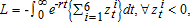 and that of gain is
 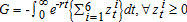 .
.
We compute the proportion, s = L/G. This is the proportion by which the size of the free block provided to the gainers is reduced.
Inasmuch as the free blocks are initially set to balance the budget within each period, additional compensatory transfers imply that the water authority will run a deficit in early periods when net compensation is positive. The principle of benefit taxation requires these to be paid by future beneficiaries, as if a bond issue is created to finance compensation. That is, compensation in period t will require borrowing,  with a present value of:
  . Repayment, Rt, in period t is given by:
  with a present value of
  Thus, we have an intergenerationally balanced budget when we set s = L/G.
Compensation in the Honolulu Case
In Honolulu, the gains (G) are computed to be $441 million and the losses (L) are $34 million (or 7.7% of the gains) in present value terms. To compensate the losers, we reduce the revenue returned to the welfare-gaining users by 7.7% (s = 34/441 = 0.077) and increase the size of the free block just enough to compensate the welfare-losing users. The total present value of the borrowing is $34 million. The borrowing and repayment streams are shown in figure 2(e).
The size of the free block to provide compensation and to return the surplus revenue is given in figure 2(d), and at selected intervals, in table 2, panel (h). The size of the free block is now initially larger for higher-elevation categories, because they are losing larger welfare by switching to efficiency pricing and need larger compensation. Over time, the free-block size increases for all categories, until the year 57 when status quo pricing would require the use of the backstop, and efficiency pricing that avoids the need for backstop is welfare superior. Thus, the size of the free block falls in year 57 when all users become gainers and do not need to be compensated. After this fall, the size of the free block continues to grow as the revenue collected from efficiency pricing increases and is returned to the users.
Alternate Compensation Plans
Intergenerational lump-sum transfers can take a variety of alternative forms and still satisfy the requirement that the pricing reform be Pareto-improving. Full compensation of each loser in each period simply provides a transparent guarantee that no one will be made worse off and, therefore, increases the chances of political feasibility of efficient management. Lower transfers are conceivable that may still compensate and/or satisfy losers. One way to lower the necessary transfers would be to consider gains that losers may make in future periods, either by living long enough or by enjoying the prospects of bequeathing to their heirs. Another is to account for capital gains in accordance with the capitalization of lower future water prices in property values. Also, if the higher-elevation users are wealthier, as is generally understood to be the case in Honolulu, they may not be sufficiently motivated to oppose the reform that causes small losses in their welfare. Then it might be possible to reduce compensation to these users, thus enhancing vertical equity without jeopardizing political feasibility. Designing reduced compensation plans based on such considerations, however, is likely to be administratively costly due to the information and other requirements involved.10
In addition, it would be unrealistic to think that the above factors can entirely remove the need for compensation. User resistance can still occur. Indeed, a proposed price increase in Hawaii was abandoned due to resistance by water users. In the year 2000, a very small increase of five cents per thousand gallons was proposed as an addition to Hawaii House Bill number HB2835 through Senate Standing Committee Report number 2919. After a prolonged public debate, the increase could not pass and was excluded from the final version of the bill approved in the House-Senate Conference (Conference Committee Report number 152, see Hawaii State Legislature, Archives).
Using the welfare gains from pricing reform to compensate the losers is one way to divide the gains. The financing mechanism discussed above allows for other ways to divide the welfare gains among users. Such reassignment of gains may, in some cases, become necessary. For instance, in year 57, when compensation is no longer needed, there is a discontinuous fall in the size of the free block. If users at the time do not approve of this decrease in the quantity of free water received, they could lobby against its reduction, creating a problem of dynamic inconsistency in block size choice. Since after year 60, the free block increases back to a size larger than it is in year 56, it is possible to reduce post-year 60 block size and use the money to keep the free-block size constant between year 56 and year 60. In other words, some of the welfare gains originally assigned to users after year 60 can be reassigned to users between year 56 and year 60. Concepts of gains division from cooperative game theory, for example, the Shapley value (Shapley 1953), the nucleolus (Schmeidler 1969), and the core's centroid (Arce and Sandler 2001), can be applied to derive other ways to assign welfare gains across users.
Conclusions
Pricing (or quantity) reforms intended to improve the efficiency of water allocation over time and space may be politically infeasible. This article provides a compensatory mechanism that renders efficiency pricing Pareto-improving. An inframarginal free block is used for two purposes. First, it is used to return the revenue surplus generated by full marginal cost pricing (including marginal user cost). Second, by lowering the block size for winners and increasing it for losers, the free block is used to compensate consumers who would lose from switching to efficiency pricing even with the budget-balancing free block. Status quo pricing favors current versus future consumers, especially those in higher elevations who are cross-subsidized by low-elevation consumers. But losses from switching to efficiency pricing are sufficiently small so that reducing gains of winners by only 7.7% provides sufficient revenue to compensate for losses in each period.
Total welfare gains from efficiency pricing are estimated to be 6.2% compared to the status quo case. These gains are large relative to those found by studies of situations with smaller demand growth and linear extraction costs. On the other hand, our results show smaller welfare gains in comparison with some studies that find a higher initial efficiency price of water and posit an even higher demand growth than in the Honolulu case.
By decomposing the sources of welfare gains, we find that the relative contribution of spatial and temporal optimization depends on which comes first. In the Honolulu case, if spatial optimization is undertaken without temporal optimization, the gains are relatively small (about $5 million). On the other hand, if temporal optimization is undertaken first (yielding $227 million), the additional gains from spatial optimization are about $180 million. Intuitively, conserving water by spatial reallocation is somewhat futile if much of the water saved thereby is wasted through aggregate overconsumption.
Temporal efficiency generates welfare gains by delaying aquifer exhaustion and the resulting need for expensive backstop technology. As such, the gains start at the time when status quo management would have resulted in the use of the backstop. Before this time, temporally efficient management causes welfare losses due to the higher efficiency prices. The gains from efficient temporal and spatial management in Honolulu are $441 million and the losses are $34 million (or 7.7% of the gains) in present value terms.
The intertemporal transfer mechanism presented in this article can be modified in order to increase or decrease transfers from winners to losers. The compensation scheme discussed ensures that there are no losers in any period, so that Pareto-improvement leads to political feasibility. In cases where political feasibility can be achieved with smaller or larger compensation, or when equity concerns other than political feasibility require a different compensation regime, the transfers can be adjusted accordingly.
Designing spatial and intergenerational compensation to render economic reforms Pareto-improving may have applications in other contexts. One such application relates to the common problem of reallocating water from agricultural to urban uses where governments are precluded from reform by concerns about equity and political feasibility. The Pareto-improving pricing reforms discussed here can be directly applied in that context as well, by giving farmers a free block or lump-sum payment sufficient to compensate them for paying efficiency prices at the margin. As in our scheme, these payments would be financed through benefit taxation, perhaps requiring debt issuance to facilitate future winners compensating current losers. More generally, the compensation methodology described can be applied where policy reforms are welfare improving in the long run but are blocked by clearly identifiable near-term losers.