Volatility linkages of the equity, bond and money markets: an implied volatility approach
I wish to thank Tim Brailsford, Tom Smith, Bill Schwert, Robert Faff, Jeff Fleming, Chris Kirby, Barbara Ostdiek, an anonymous referee, my colleagues at the UQ Business School (UQBS) and the Australian National University (ANU), and seminar participants at Tsinghua University, ANU and York University for helpful suggestions. Financial support and research assistance from UQBS are gratefully acknowledged.
Abstract
This study proposes an alternative approach for examining volatility linkages between Standard & Poor's 500, Eurodollar futures and 30 year Treasury Bond futures markets using implied volatility from the three markets. Simple correlation analysis between implied volatilities in the three markets is used to assess market correlations. Spurious correlation effects are considered and controlled for. I find that correlations between implied volatilities in the equity, money and bond markets are positive, strong and robust. Furthermore, I replicate the approach of Fleming, Kirby and Ostdiek (1998) to check the substitutability of the implied volatility approach and find that the results are nearly identical; I conclude that my approach is simple, robust and preferable in practice. I also argue that the results from this paper provide supportive evidence on the information content of implied volatilities in the equity, bond and money markets.
1. Introduction
Investors who invest in more than one market are exposed to more than one kind of market volatility risk. Hence, examining the linkages of financial market volatilities is important for investment and risk management decisions.1 In light of this, researchers, such as Fleming et al. (1998), have examined the volatility linkages across stock, bond and money markets.2 Based on Tauchen and Pitts (1983) and Ross (1989), Fleming et al. (1998) develop a multivariate speculative trading model and generate moment conditions from that trading model. The market volatility correlations between stock, bond and money markets are estimated using a bivariate generalized method of moments (GMM) system directly.
Although the approach of Fleming et al. (1998) is well regarded among researchers, their volatility proxies are in nature historical and their method is too complicated for practical purposes. The GMM they use requires significant programming effort and is somewhat costly to implement. Indeed, as can be demonstrated, it is quite difficult for most people to interpret and apply their GMM approach. As a result, this approach remains highly academic rather than practical. From this perspective, an alternative method that is both simple and reliable in examining volatility and informational linkages across financial markets needs to be found. The current study seeks to find such a method.
The critical factor in examining market volatility linkages is the measure of market volatility. An alternative to the GMM approach of Fleming et al., which is based on historical volatility, is to use implied volatility. Implied volatility is frequently argued to be more effective for approximating the true market volatility and forecasting future market movement.3 Based on this, a volatility and informational correlation study can be facilitated by using implied volatility calculated from option prices, instead of extracting the historical volatility information from historical returns. This alternative is expected to provide a better measure of volatility and information linkages.
I propose to directly estimate market volatility linkages between the Standard & Poor's (S&P) 500 index market, the Eurodollar futures market and the 30 year US Treasury Bond futures market using the implied volatility series. There are at least two advantages of this approach: first, implied volatility data for the three proposed markets is readily available and as indicated above the idea behind implied volatility is much more comprehensive and straightforward; and, second, with the readily available implied volatility data it is easier to examine market linkages using common statistical techniques.
I find that using implied volatility in studying financial market linkages is both feasible and simpler. Other notable advantages include easy detection of spurious correlation effects as well as facilitating the study of time series properties of the market volatility and information flow process. It is a robust alternative to the GMM approach of Fleming et al. (1998) and provides quick and easy assessment of the strength of financials markets linkages.
The present paper is organized as follows: Section 2 discusses the implied volatility data and estimates the market linkages between the equity, money and bond markets using implied volatility. Section 3 replicates the GMM approach of Fleming et al. (1998) as a comparison and a substitutability check to show the effectiveness and feasibility of the implied volatility approach, and Section 4 offers a summary and conclusion of the study.
2. Implied volatility linkages across equity, money and bond markets
2.1. Implied volatility calculation
The current study proposes to use implied volatility to assess volatility linkages across financial markets. One of the key questions is which implied volatility to use. Beckers (1981) shows that using only at-the-money (ATM) options is preferable to other weighting schemes in deriving implied volatility from option prices. However, weighted average implied volatility has also been used to construct volatility indexes.4 The general conclusion from most of the previous studies is that ATM option implied volatility is as good as a weighted-average implied volatility in predicting future volatility.5 Furthermore, ATM options are the most liquid options and, therefore, the least likely to suffer from non-simultaneity problems. Jorion (1995) also suggests that using the arithmetic average of the implied volatilities from ATM call and put alleviates some of the measurement problems derived from misspecification of the option pricing models. Ederington and Guan (2000) also argue that averages forecast (from just a few ATM options) slightly better than the broader weighted averages (from a wide range of option classes) of implied volatilities in terms of forecasting ability for the future market volatility.
In view of these alternatives, implied volatility from ATM options is used in the present study to assess market volatility linkages. Following Jorion (1995), I use the average of call and put implied volatility to alleviate the misspecification problems. To be more specific, I use the Chicago Board Options Exchange's (CBOE) new volatility index (VIX) for the S&P 500 index market, and interpolated implied volabilities which are calculated as average of ATM call and put implied volatilities for the Eurodollar futures market and for the 30 year US Treasury Bond futures market.
2.2. Sample
The new VIX daily continuous series are obtained from the CBOE and the ATM call and put option daily continuous implied volatility series for the Eurodollar futures and the 30 year US Treasury Bond futures markets are obtained from the Commodity Research Bureau. In calculating the ATM interpolating implied volatility, the nearest two options series ATM are used: one just above and one just below the underlying price; and the implied volatilities I use in the present study are averages of the call and put implied volatilities in the Eurodollar and the Treasury Bond markets. My sample spans a 10 year period from 5 January 1998 to the end of December 2007, and contains 2606 daily observations. Table 1 presents summary statistics for the three implied volatility series.
| Panel A: Summary statistics | ||||||
|---|---|---|---|---|---|---|
| Mean | Median | SD | Skewness | Kurtosis | AR(1) | |
| VIX* | 0.1973 | 0.1891 | 0.0687 | 0.7221 | 3.0196 | 0.9515 |
| σimp.Eurodollar | 0.1943 | 0.1731 | 0.1387 | 0.9657 | 3.6193 | 0.9026 |
| σimp.T–bond | 0.0957 | 0.0932 | 0.0263 | 0.6191 | 4.2142 | 0.9137 |
| Panel B: Correlation matrix | |||
|---|---|---|---|
| VIX* | σimp.Eurodollar | σimp.T–bond | |
| VIX* | 1.0000 | 0.5961 | 0.4759 |
| σimp.Eurodollar | 0.5961 | 1.0000 | 0.6024 |
| σimp.T–bond | 0.4759 | 0.6024 | 1.0000 |
- * VIX converted to %. This table gives summaries for the three implied volatility series in the study (2606 daily observations over the sample period from 5 January 1998 to 31 December 2007). VIX is the CBOE implied volatility index ‘VIX’ calculated with the new method for the Standard & Poor's 500 index market; σimp.Eurodollar is the interpolated at-the-money option implied volatility, which is calculated as average of call and put implied volatility for the 3 month Eurodollar futures market; σimp.T–bond represents the interpolated at-the-money option implied volatility, which is calculated as average of call and put implied volatility for the 30 year US Treasury Bond futures market. AR(1) is the first-order autocorrelation coefficient of the implied volatility series. SD, standard deviation.
One of the most notable features of the three implied volatility series is that the first order autocorrelation coefficients are all close to unity (Panel A). This suggests that implied volatilities in the equity, bond and money markets are highly persistent. Although the unit root tests reject the hypothesis that the implied volatilities have unit root, a high level of first order autocorrelations might raise the concern that a correlation study between the series may be susceptible to spurious effects. Panel B reveals the correlation matrix between the implied volatility series in the equity, bond and money markets at the daily level over the past 10 years. The common sample correlation matrix implies that there is a high level of co-movement between the equity, bond and money markets, with the equity–money and the money–bond pairs having a correlation coefficient around 0.6, and the equity–bond pair a correlation coefficient around 0.5. One of the concerns following the preliminary examination is whether the high correlations between the implied volatilities are obtained due to the high persistency of the implied volatility series; or, in other words, are the results spurious? I address this concern below.
2.3. Spurious correlation examination
The highly persistent implied volatilities in the current study raise concern over the spurious correlation effects. Spurious correlation was first investigated by Granger and Newbold (1974). Philips (1986) further develops the concept and techniques. The recent literature on spurious regression points out that the use of persistent independent variables can lead to spurious regression results when the dependent variable is also at least partially persistent, as error terms in the regression equation inherit autocorrelation from the persistent dependent variable (Ferson et al., 2003). This autocorrelation in the error term leads to biased standard error estimates and can therefore indicate a significant relationship where none exists. Granger et al. (2001) boost our understanding of spurious regression by examining it with a stationary time series. They argue that spurious regression occurs not only with pairs of independent unit root processes but also with positively autocorrelated autoregressive series or long moving averages. And it occurs regardless of the sample size and for various distributions of the error terms. Hence, my volatility correlations are susceptible to spurious effects due to the strong persistence of the implied volatility series. Below I propose a means for detecting and controlling for these effects for the correlations between implied volatility in the three markets.
In computing correlations between implied volatilities in the equity, bond and money markets, I carry out a simple correlation analysis by running the following regression:
σit = α + βσjt + ɛt,
()where σit is the time t natural log implied volatility in market i; σjt is the time t natural log implied volatility in market j; and α is a constant and ɛ is the error term. The correlation between the two markets is the root to the R2 of this regression with its sign determined by the sign of beta, the slope parameter. To detect the spurious effect, I set up a Monte Carlo simulation procedure. It provides the cut-off R2 that would be obtained from a regression for which the dependent and independent variables are uncorrelated but have the same autocorrelation properties as the actual data; hence, taking account of the potential for spurious regression (see also Foster et al., 1997; Ferson et al., 2003). To obtain the cut-off R2 using the simulation, the moments and the serial correlation properties of the regression variables are first estimated for each data series. Uncorrelated dependent and independent variables with the same serial correlation properties and sample moments are then simulated for a time period equal to the sample length with the same frequency of the data in the sample. A regression is then run on these simulated series. The process is repeated 1000 times, and the R2's and adjusted R2's are recorded for each regression and ranked from lowest to highest. The 95th percentile cut-off R2 is reported and compared to the actual R2 for the same regression run using the original data.6
Table 2 reports the implied volatility correlation estimates and the spurious regression simulation results for the three markets.7 Panel A of Table 2 gives the moments and the first-order autocorrelation coefficients for the three log implied volatility series; Panel B gives the spurious regression simulation 95th percentile cut-off levels, the regression R2's with the empirical p-values based on simulations, and the estimated correlation coefficients between the market implied volatilities.
| Panel A: Log implied volatility summaries | |||
|---|---|---|---|
| S&P 500 | Eurodollar | 30 year Treasury Bond | |
| µ | –1.6815 | –1.9287 | –2.3865 |
| σ | 0.3422 | 0.6162 | 0.2991 |
| ρ1 | 0.9486 | 0.9223 | 0.9025 |
| Panel B: Spurious regression effect diagnostics | |||
|---|---|---|---|
| S&P 500 (i)/Eurodollar (j) | S&P 500 (i)/30 year Treasury Bond (j) | Eurodollar (i)/30 year Treasury Bond (j) | |
| 95% | 0.1879 | 0.1148 | 0.1526 |
| R 2 | 0.3556 | 0.2222 | 0.3481 |
| (p-value) | 0.0382 | 0.0415 | 0.0358 |
| ρi,j | 0.5963 | 0.4714 | 0.5901 |
- This table presents the results for the equity, money and bond market implied volatilities correlations. Panel A gives the description of each of the three natural log implied volatility series (2606 observations over the sample period from 5 January 1998 to 31 December 2007). µ is the mean of natural log of the implied volatility; σ is the standard deviation of the series; and ρ1 is the first-order autocorrelation. Panel B gives the correlation estimations and spurious regression Monte Carlo simulation 95 per cent cut-off levels using 1000 simulations for each pair of the market correlations. R2 is the R2 of the reported regressions of the form ln(i) = a + βj ln(j), where i and j represent implied volatility in market i and j respectively; the p-values are the associated empirical p-values for the R2's, which are calculated as the proportion of the simulated R2's exceeding the calculated R2's in the 1000 simulations; ρi,j is the correlation of i and j, which is the square root to the R2, and the sign of the correlations are determined by the sign of the coefficient of ln(j), βj. S&P 500, Standard & Poor's 500.
From Panel A, the means are all negative; the first-order autoregression coefficients are obtained by ordinary least-squares regression with Heteroscedasticity and Autocorrelation Consistent (HAC) standard errors. Again, I have a highly persistent implied volatility series. From Panel B, the result indicates that there is a strong linkages across equity, bond and money markets as there are strong positive correlations between the implied volatilities of the markets. The calculated R2 for the equity and money market is 0.3556, which is greater than the 95 per cent cut-off level of 0.1879. The associated empirical p-value is significant at the 5 per cent level (an empirical p-value of 0.0321), indicating that the spurious regression hypothesis is rejected for the equity and money markets correlation regression. The correlation coefficient between the two markets gives a value of 0.5963, which is the positive root to the R2. The correlations between the remaining two pairs of markets are also positive and robust in regard to the spurious correlation effect. At the 5 per cent level, the hypothesis that correlations between the equity–bond and the bond–money markets are spurious can be rejected. The obtained correlation coefficients across the three markets in Table 2 are nearly identical to those obtained in Table 1, where the simple correlation coefficients are obtained with the common sample. Therefore, I demonstrate that the simple correlations between the implied volatilities in the three markets are robust to spurious effects.
The proposed implied volatility approach now needs to be tested for its substitutability for established methodologies. I use the GMM approach of Fleming et al. (1998) to do this test, as their approach is widely regarded as consistent and robust.
3. Substitutability check
3.1. The GMM approach to estimating the three market volatility linkages
The GMM approach for studying market volatility correlations used by Fleming et al. (1998) is based on the relation between volatility and information flow (Ross, 1989). Using this approach, they begin by developing a model of speculative trading that formalizes this information and volatility relation and generates predictions about how information creates cross-market correlations. This approach assumes that daily returns are generated by the joint stochastic process below:
 ()
() ()
() ()
()where  ; ɛik,t denotes the incremental return produced by event i; Ik,t is the number of information events that impact the market k on day t; σɛ,k is standard deviation of ɛik,t; uk,t, and zk,t are independent, zk,t ~ iid. N (0, 1); and uk,t is iid, with mean zero and variance
  . The unpredicted component of returns is defined as rk,t = Rk,t – µk,t. The autocorrelation of rk,t is zero at all lags, but there can be a substantial degree of high order serial dependence. Therefore,
 ()
()Since zk,t is normally distributed with mean zero and variance one, the mean and variance of  are –1.27 and 4.93 (Abramowitz and Stegun, 1970). If
  is defined, the transformed system can be obtained:
 ()
()where  is mean zero and variance 4.93, and independent of hk,t. Therefore, moment restrictions on yk,t that form the basis for estimation of the model are:
 ()
()This generates the moment conditions in one single market for univariate estimation. Similarly, the bivariate estimation moment conditions can also be derived. The moment conditions for bivariate estimation can be stated as:
 ()
()where τ = 1, 2, 3 . . . , l, counts the number of autocorrelation restrictions used in the estimation, and  = 4.93. To obtain the GMM parameter estimates, gT(θ)′Ŝ−1gT(θ) needs to be minimized, where
  , and Ŝ is a consistent estimate of the GMM covariance matrix. The choice of Ŝ adjusts for conditional heteroscedacity and autocorrelation using Parzens weights and the Andrew (1991) method of bandwidth selection. The cross-market correlations are estimated by fitting the above bivariate GMM moment systems three times, pairing equity–money markets, equity–bond markets and money–bond markets. In the equation system above, i and j subscripts denote, respectively, equity and money, equity and bond, money and bond. ρh,ij is the correlation between hi,t and hj,t; and ρξ,ij is the correlation between ξi,t and ξj,t. The first six moment conditions are for univariate estimation for the two markets in each pair. We have 2(l + 2) equations and six unknowns [three for each market,
 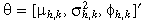 , k = i,j]. There are 2l + 1 cross-market equations with two unknowns in the remaining moment conditions, which makes 4l + 5 equations with eight unknowns in the joint system.
After the GMM estimation moment conditions are determined, we implement the GMM estimation procedures in obtaining the cross-market volatility correlations between the equity, money and bond markets. As in Fleming et al. (1998), I use the S&P 500 futures contracts traded on the Chicago Mercantile Exchange (CME), the 30 year Treasury Bond futures contracts traded on the Chicago Board of Trade (CBOT), and the CME's Eurodollar futures contracts as proxies for the equity, bond and money markets. The futures data are the daily closing prices for each contract, obtained from DataStream, covering the period from 5 January 1998 to 31 December 2007.
To maintain a uniform measurement interval across markets, the days when any of the three markets is closed are excluded from the sample. The daily returns for each market are measured as the log of price relatives, using closing prices for the nearest-to-maturity contract. To generate the continuous series of returns, I switch to the new contract as the nearby contract approaches maturity. On the day of each switch, I compute the return using the current and previous day's prices for the new contract. This procedure yields 2578 return observations in each of the three markets.
To construct the data (yk,t) needed for the GMM estimation, the following procedure is followed. First, remove the return seasonality by using the residuals, rk,t, from a regression of the raw returns on a set of six dummy variables: one for each weekday, and one for the days following a market holiday; the market holiday information is obtained from the CBOT and the CME. Second, remove the volatility seasonality by regressing  on a constant, one dummy variable for Monday, and one dummy variable for the days following the market holidays. The yk,t series is finally obtained by subtracting E[
 ] or –1.27 from the sum of the intercept and residuals of the regression in the second step above. Equations (9) to (11) illustrate the three steps of the procedure.
 ()
() ()
() ()
()where Di are dummy variables: D1 and D6 stand for Monday dummy and Holiday dummy, respectively.
The GMM procedure yields a direct test for specification error in the form of an over identifying test statistic (Hansen, 1982). Choosing a suitable value for l, the number of autocorrelation restrictions used in the estimation, involves conflicting considerations. The empirical evidence indicates that the daily volatility of returns is highly persistent, suggesting that a large value of l may be appropriate. But maintaining a small number of moment conditions typically reduces the bias of the parameter estimates, and minimizes the possibility of obtaining an ill-conditioned weighting matrix. Hence, I estimate the specification of the system for l equal to 1, 10, 20, 30 and 40. In general, the results are insensitive to the choice of l. Following Fleming et al. (1998), I report the results for the 40 lag case.
Table 3 provides the results from the GMM estimation. The mean of hk,t is largest in the equity market and smallest in the money market. This ordering indicates stock returns are more volatile than bond returns, which in turn are more volatile than the Eurodollar returns. However, note that the variance of hk,t is largest for the money market at 0.81945 or 0.81424, and smallest for the equity market; this may seem counterintuitive, but recall that  is the variance of ln(Ik,t), the information flow. Hence, when the mean of Ik,t is very small, the log transformation yields an hk,t series that is highly variable. In fact, if we assume that hk,t is normal and use its moment generating function to compute the variance of Ik,t implied by each of these estimates, the variance is largest for the equity market, followed by bond and then money market. The over-identifying test statistics reveal little evidence of misspecification for any of the three GMM bivariate system estimations. The estimated parameter that is of greatest interest in the system is the correlation of the log volatility between markets, ρh,ij, which reflects the linkages between market information. The estimate for the correlation of the equity–money pair is 0.61318, with standard error 0.05811; the estimate for the equity–bond pair is 0.49122, with standard error 0.19522; and the estimate for the money–bond pair is 0.60301, with standard error 0.06852. Because all the standard errors are small, the correlations are relatively precisely estimated.
| Parameter | Equity(i)/Money(j) | Equity(i)/Bond(j) | Money(i)/Bond(j) | |||
|---|---|---|---|---|---|---|
| Coefficient estimates | Standard error | Coefficient estimates | Standard error | Coefficient estimate | Standard error | |
| µh,i | –11.65256 | 0.09852 | –12.08543 | 0.12254 | –16.32566 | 0.09764 |
 |
0.73921 | 0.06261 | 0.65699 | 0.15131 | 0.81424 | 0.04529 |
| φh,i | 0.95022 | 0.00382 | 0.92362 | 0.01653 | 0.91959 | 0.00597 |
| µh,j | –16.73678 | 0.07956 | –12.54197 | 0.08589 | –14.14829 | 0.05816 |
 |
0.81945 | 0.06118 | 0.79215 | 0.22106 | 0.73965 | 0.10985 |
| φh,j | 0.92051 | 0.00236 | 0.90156 | 0.13543 | 0.89125 | 0.05293 |
| ρh,ij | 0.61318 | 0.05811 | 0.49122 | 0.19522 | 0.60301 | 0.06852 |
| ρξ,ij | 0.22993 | 0.06332 | 0.20558 | 0.03122 | 0.37529 | 0.04116 |
| J-statistic | 128.2356 | 102.3258 | 116.21591 | |||
| p-value | 0.72365 | 0.79865 | 0.82766 | |||
-
This table reports the generalized method of moments parameter estimates and over-identifying test statistics (J-statistic) for the bivariate model of the log volatility (hk,t) in the equity, money and bond markets. The estimation procedure uses the moment conditions implied by the model for seasonally adjusted, log squared returns (yk,t) to estimate the mean, variance and AR(1) parameters of the log volatility processes. The bivariate estimation also provides the estimates of the correlations between the volatilities (ρh,ij) and between the disturbance terms (ρξ,ij) in market i and j. This table reports the coefficients estimates and standard errors for each model based on the lag length of 40, as well as the J-statistics which, under the model, are distributed
 ; the sample period is from 5 January 1998 to 31 December 2007 (2578 daily observations).
Recall that in the previous section the market volatility correlation for the equity–money pairing is about 0.5963; the correlation for the equity–bond pairing is 0.4714; and the correlation for the money–bond pairing is 0.5901. Comparing these with the GMM estimations results above we can see that they are nearly identical. Therefore, we have nearly the same results from the two approaches regarding the same issue. Because the GMM approach of Fleming et al. is tested to be consistent and robust, I believe that results from my implied volatility approach are also consistent and reliable.
3.2. Comparison of the two approaches
Comparing the two approaches, I note that the GMM approach is based on a theoretical analysis of the trading process and represents a way to embed a stochastic volatility specification within a rational expectations framework. The implied volatility approach, in contrast, needs no trading model as a base for deriving the volatility series and information flow process. In this approach, the volatility series are obtained directly from the market option prices, instead of being generated from the returns of the underlying financial assets. This way of generating volatilities incorporates market information concealed in the option prices and is one major difference between the two approaches.
The GMM approach also needs sophisticated statistical analysis skills in programming and interpreting the estimations. The implied volatility approach, in contrast, uses common statistical techniques to implement and interpret the correlation analysis and, hence, is much simpler for practical purposes. The fact that the same results are achieved from the two approaches further highlights the advantage of the implied volatility approach. In the implied volatility approach, the time series structure of the market volatility as well as market information flow can be easily assessed and there is no need to assume the structure of the information flow process as in the GMM approach; hence, greatly improving the credibility of the results. On the basis of the current study, I suggest that volatility and information linkages between financial markets can, alternatively, be examined with the implied volatility approach. I argue that this approach is simple and robust and, hence, represents a more practical way than other methods.
4. Conclusion
The present study examines the market volatility linkages across the equity, money and bond markets using implied volatility. A simple correlation analysis in the three markets accounting for spurious correlation effects is performed. The results indicate that the correlations between equity, bond and money markets are positive, strong and robust. To check the substitutability of the proposed implied volatility approach, I replicate the GMM approach of Fleming et al. (1998) for the three markets over the same sample period and obtain nearly identical results. The implied volatility approach is then concluded to be consistent, practical and preferable in assessing the market volatility and informational linkages.