Inference without significance: measuring support for hypotheses rather than rejecting them
Abstract
Despite more than half a century of criticism, significance testing continues to be used commonly by ecologists. Significance tests are widely misused and misunderstood, and even when properly used, they are not very informative for most ecological data. Problems of misuse and misinterpretation include: (i) invalid logic; (ii) rote use; (iii) equating statistical significance with biological importance; (iv) regarding the P-value as the probability that the null hypothesis is true; (v) regarding the P-value as a measure of effect size; and (vi) regarding the P-value as a measure of evidence. Significance tests are poorly suited for inference because they pose the wrong question. In addition, most null hypotheses in ecology are point hypotheses already known to be false, so whether they are rejected or not provides little additional understanding. Ecological data rarely fit the controlled experimental setting for which significance tests were developed. More satisfactory methods of inference assess the degree of support which data provide for hypotheses, measured in terms of information theory (model-based inference), likelihood ratios (likelihood inference) or probability (Bayesian inference). Modern statistical methods allow multiple data sets to be combined into a single likelihood framework, avoiding the loss of information that can occur when data are analyzed in separate steps. Inference based on significance testing is compared with model-based, likelihood and Bayesian inference using data on an endangered porpoise, Phocoena sinus. All of the alternatives lead to greater understanding and improved inference than provided by a P-value and the associated statement of statistical significance.
`Null hypothesis testing in the statistical sciences is like protoplasm in biology; they both served an early purpose but are no longer very useful’
Introduction
David Anderson’s comment is part of a long history of criticism of null hypothesis significance testing (NHST) by statisticians and statistically minded biologists. Some colorful comments about NHST procedures are that they are ‘not a contribution to science’ (Savage 1957), ‘a serious impediment to the interpretation of data’ (Skipper et al. 1967), ‘worse than irrelevant’ (Nelder 1985), ‘difficult to take seriously’ (Chernoff 1986), and ‘completely devoid of practical utility’ (Finney 1989). The long and intense criticism does not seem to have had much effect in ecology. Although use has declined slightly (Fidler et al. 2006; Hobbs & Hilborn 2006), NHST and its associated P-value are currently used in over 90% of papers in ecology and evolution (Stephens et al. 2006).
NHST is based on positing that a certain condition (the null hypothesis) is true and then calculating the probability (the P-value) of the observed data, or of unobserved data more extreme, given the hypothesis and the probability model.1 The basic idea is that an improbable outcome (small P) is reasonable cause to question the validity of the null hypothesis. The assumption of a null hypothesis leads to the burden-of-proof issue, because the null hypothesis remains the accepted condition unless and until data indicate that it should be rejected. In the context of conservation or wildlife management, where data are often limited, the requirement to disprove a null hypothesis of no effect or no impact can have non-precautionary implications (Peterman & M’Gonigle 1992; Taylor & Gerrodette 1993; Dayton 1998; Brosi & Biber 2009).
As currently used, NHST is a combination of ideas developed in the 1920s and 1930s, primarily by Fisher (1925) and Neyman & Pearson (1933). Actually, these and other statisticians had substantially different views about the nature and role of statistics in the scientific process. There were vigorous disagreements at the time (Goodman 1993; Inman 1994; Salsburg 2001) and it is doubtful that any of them would approve of NHST as it is practiced today. Fisher’s idea was that the P-value was an ‘aid to judgment’ about the truth of a hypothesis. A small P-value meant that the data did not support the hypothesis, but Fisher was not dogmatic about a 0.05 cutoff for significance (see Hurlbert & Lombardi 2009 for changes in Fisher’s thinking), nor did he view the outcome of any single experiment as decisive. Neyman and Pearson, on the other hand, explicitly framed the problem as a decision between two competing hypotheses. Fisher’s P-value was a flexible measure of evidence, whereas the Neyman–Pearson test was a rule for behavior which would minimize the rate (or frequency, hence the term ‘frequentist’) of incorrect decisions. The modern hybrid NHST combines these ideas by identifying Fisher’s P with the Neyman–Pearson Type I error rate α. The two methods are fundamentally incompatible, and the result is ‘a mishmash of Fisher and Neyman-Pearson, with invalid Bayesian interpretation’ (Cohen 1994). Their combination ‘has obscured the important differences between Neyman and Fisher on the nature of the scientific method and inhibited our understanding of the philosophic implications of the basic methods in use today’ (Goodman 1993).
This paper makes three points: (i) that NHST is widely misused and misunderstood; (ii) that even when properly used, NHST is only marginally informative for most ecological data; and (iii) that better methods of inference are available. The first two points are covered relatively briefly, as the problems with NHST have long been well described.2 However, many of the papers are in the statistical, medical and social science literature and may not be familiar to ecologists. An excellent paper on ‘the insignificance of significance testing’ for ecologists is Johnson (1999) (see also Yoccoz 1991; McBride et al. 1993; Ellison 1996; Cherry 1998;Germano 1999;Anderson et al. 2000;Läärä 2009). The third point is illustrated by working through a specific example, showing that alternatives to NHST can give greater insight and understanding of data.
As in any branch of science, new and improved statistical methods are constantly being developed. Ecologists would not use 80-year-old genetic or physiological techniques when more powerful and useful methods are available. Why don’t we apply the same standards when drawing conclusions from our data?
Misuse and misunderstanding of NHST
Probably the most pervasive and serious misuse of NHST is to interpret a P-value as the probability that the null hypothesis is true. A small P-value, particularly P < 0.05, is taken to mean that the null hypothesis is false, or at least likely to be false. A variant of this misinterpretation is to regard a non-significant result as confirmation of the null hypothesis. Thus, after finding that P > 0.05, a common conclusion is something like ‘There is no difference’ or ‘There is no effect’. Another variant, when there is a clear alternative hypothesis, is to interpret 1 − P as the probability that the alternative hypothesis is true. Yet another variant is that if the null hypothesis is rejected, the theory or idea that motivated the test must be true.
In one form or another, all of these misuses involve regarding the P-value as a statement about the probability of a hypothesis being true. But P cannot be a statement about the probability of the truth or falsity of any hypothesis because the calculation of P is based on the assumption that the null hypothesis is true. P is the probability of data (or of data more extreme) conditional on a hypothesis, not the probability of a hypothesis conditional on data. This may sound like statistical double-talk but the difference is fundamental. The probability that I will encounter a certain species, given that it is rare in the study area, is quite different from the probability that the species is rare in the area, given that I have encountered it.
The common misinterpretation of P as the probability that the null hypothesis is true is appealing because it seems logical. Consider the following:
If the hypothesis is true, this observation cannot occur.
This observation has occurred.
Therefore, the hypothesis is false.
This is a valid syllogism in deductive logic called modus tollens, or denying the consequent. The logic of NHST is similar, but the statements are probabilistic:
If the null hypothesis is true, this observation is unlikely to occur.
This observation has occurred.
Therefore, the null hypothesis is likely to be false.
The structure of the NHST argument is the same, and the logic seems reasonable. But it is invalid. Why? Because we have moved from the black-and-white of deductive logic to the grays of probabilistic inference, and the rules are different. An example will show the fallacy:
If this person is a chemist, he/she is unlikely to win a Nobel Prize in chemistry.
This person has won a Nobel Prize in chemistry.
Therefore, this person is unlikely to be a chemist.
The first statement, while true, is about the proportion of chemists who win Nobel Prizes. The validity of the conclusion, however, depends on the proportion of Nobel Prize winners in chemistry who are chemists, and neither the data (the second statement) nor the assumptions (the first statement) say anything about that. We are attempting to make a statement about the probability of truth of a statement (that the person is a chemist) using a framework of deductive logic when the situation calls for probabilistic reasoning. In the language of conditional probabilities, we want the probability of being a chemist conditional on winning a Nobel Prize in chemistry, not the probability of winning a Nobel Prize conditional on being a chemist.
The illogic of NHST has been pointed out many times before (e.g.Berkson 1942; Rozeboom 1960; Bakan 1966; Oakes 1986; Cohen 1994; Royall 1997; Goodman 1999; Trafimow 2003). Despite the faulty logic, the NHST pseudo-syllogism is alluring and continues as one of the ‘fantasies of statistical significance’ (Carver 1978). A further complication is that there are situations where the logic seems to work perfectly well. Substitute ‘this is a fair coin’ for ‘this person is a chemist’ and ‘10 “heads” in a row’ for ‘win a Nobel Prize’ in the argument above, and everything can seem fine.
Aside from its logical problems, NHST has a subtly corrosive effect because it permits lazy analysis and impedes clear thinking. NHST has become so ingrained and automatic that it is carried out by researchers and is often required by journal editors with little thought about what the procedure means or whether it is necessary. ‘Statistical “recipes” are followed blindly, and ritual has taken over from scientific thinking’ (Preece 1984). ‘The ritualization of NHST [has been carried] to the point of meaningless and beyond’ (Cohen 1994). Nelder (1985) decried ‘the grotesque emphasis on significance tests’, and Salsburg (1985) satirized ‘the religion of statistics’. Statistical ritual leads to publication of papers that are methodologically impeccable but contain little actual information (Guthery 2008).
For example, one result of rote use of NHST is a confusion of statistical significance and biological importance (Boring 1919; Jones & Matloff 1986). Many ecologists are familiar with the idea that important biological effects may exist but not be statistically significant in a particular study because of small sample size. Calculations of statistical power can be helpful in this situation (Gerrodette 1987; Cohen 1988; Urquhart & Kincaid 1999; Gray & Burlew 2007), but power calculations, especially post hoc, are themselves confusing, misunderstood and misused (Goodman & Berlin 1994; Steidl et al. 1997). In particular, a power calculation based on the observed data provides no more information than the P-value itself (Thomas 1997; Hoenig & Heisey 2001). Despite the general awareness of possible low power, a biological effect that is not statistically significant is often summarily dismissed as unimportant (‘Growth rate was not significantly related to temperature’) or nonexistent (‘There was no difference in mean length among groups’). Effect size may not even be reported, leaving the reader uninformed about the estimated size of the biological effect, statistically significant or not. However, lack of statistical significance does not mean lack of biological importance.
The converse can also happen – that is, biologically unimportant effects can be statistically significant if sample size is large. When samples can be obtained relatively easily and cheaply (e.g. air, water or, increasingly, genetic samples), large sample size can lead to detection of trivial differences and ultra-precautionary ‘significant’ results (McBride 2005). A colleague recently showed me a paper which examined prey size for two predators, based on a large sample of stomach contents (Fig. 1A). The authors had concluded that one predator ate larger prey than the other, based on a statistically significant difference (P < 0.001) in median prey length. Looking at Fig. 1A, does the difference in prey lengths seem ecologically significant? Can you even tell which predator eats the larger prey? The authors had lost sight of the difference between statistical significance and biological importance.
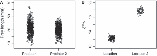
Two unthinking uses of significance tests. (A) Statistical significance is not the same as biological significance. A paper concluded that length of prey was significantly greater for Predator 1 (P < 0.001). (B) A significance test confirms the obvious. An editor required a significance test to show that the two locations had different δ15N stable isotope ratios.
A less harmful but more mindless use of NHST is to give a statistical blessing to results that don’t need it. Another colleague found a large difference in stable δ15N isotope ratios of a predator at two locations (Fig. 1B). An editor insisted that a significance test for the difference in isotope ratios between the two locations be carried out before the paper could be published. Can you believe it? Do we learn anything by assuming that δ15N values at the two locations were equal (when clearly they were not), and then calculating that P < 0.0000000000000001? (This small value is not the probability that the two locations have equal isotope values, as just explained, although we tend to think of it that way.)
Significance tests are commonly used in intermediate steps in an analysis. NHST may be used to decide whether to pool subsets of data, whether the data can be considered to follow a certain distribution (goodness-of-fit tests), and whether a parameter should be retained in an analysis or dropped because it is ‘not significant’. In nearly all such applications, lack of statistical significance is equated with the plausibility of the null hypothesis and implausibility of the alternative, when in actuality the null and alternative hypotheses were not resolvable with the data. For example, using a significance test to determine if data are normally distributed will reliably lead to the conclusion that the data are normal if sample size is small and not normal if sample size is large, an observation that led Berkson (1938) to an early criticism of NHST. In addition, multiple testing within an analysis leads to inflated Type I error rates and many false results, particularly in stepwise regression (Whittingham et al. 2006; Anderson 2008; Mundry & Nunn 2009).
The P-value is sometimes regarded as a measure of effect size, so that a small P is taken to indicate a large (‘significant’) effect. However, P depends on sample size as well as effect size, and the relationship between P and effect size can be highly non-linear even with equal sample sizes. Here is a thought experiment that shows how these can be confused. Suppose we conduct experiments designed to measure the effect of two toxins. The experiment with the first toxin has a sample size of 100 and gives P = 0.01. The experiment with the second toxin has a sample size of 10 and gives P = 0.07. Which toxin has the stronger effect? It is tempting to say the first, because P is lower and significant at the 0.05 level, and sample size is larger. Actually, however, the results indicate a stronger effect for the second because, despite the much smaller sample size, the P-value is still relatively small. With the usual assumptions of normal distributions and equal variances, the results indicate that the effect of the second toxin is q(0.07)/q(0.01) times as large as the first, where q(x) is the standard normal quantile of x. Given the difference in sample sizes, to indicate an equal toxic effect the P-value of the first experiment would have to be
  , where Φ is the standard normal cumulative distribution function. The relationships between P, sample size and effect size are not simple.
By focusing on the P-value and a sharp boundary between significance and non-significance, NHST can hinder rather than help interpretation of data. As Hoenig & Heisey (2001) conclude: ‘The indirect logic of frequentist hypothesis testing is simply nonintuitive and hard for most people to understand’.
Marginal utility of NHST
Even if NHST is understood and used properly, the results are usually not very informative for making inference with ecological data. As discussed in the previous section, NHST poses the problem in a way that does not give the answer that most ecologists need, and that most ecologists think it gives them. A P-value is the right answer to the wrong question.3
For example, provided all assumptions have been met, a P-value for the slope of a regression line indicates whether the observed relationship between the x and y variables could have occurred by chance alone. But what we need to know is how much the data support a slope of 0 versus a slope that would indicate an important effect. The NHST approach does not provide a measure of how improbable a slope of 0 is – that is, no measure of how strongly chance might be eliminated as an explanation of the data. The P-value itself, as we have seen, is not such a measure. Similarly, the Type I error rate is a measure of how frequently the wrong conclusion will be reached if the null hypothesis is true, and the Type II error rate provides a similar measure if the alternative hypothesis is true. However, there is no measure of which of these two hypotheses, the null or alternative, might be true. Further, the calculation of P and error rates depends on unobserved data. Basing conclusions on what might have been observed, but was not, does not seem the best way to proceed. What might have been observed may depend on the intentions of the investigator (Meeks & D’Agostino 1983; Berger & Berry 1988).
Fisher regarded the P-value as a relative measure of support, and inference based on P was a reasoned judgment, neither automatic nor absolute. In modern use, P is usually interpreted in an absolute sense, so that a small P, say P < 0.05, is regarded as moderately strong support against the null hypothesis, and P < 0.01 as strong support. The P-value has no such absolute meaning because it depends on the alternatives (Berkson 1938; Oakes 1986; Schervish 1996; Royall 1997). A result with P < 0.05 does not necessarily provide strong support against the null hypothesis (Edwards et al. 1963; Sterne & Davey Smith 2001). In fact, results with P = 0.05 are at most weak support, and the null hypothesis may still have substantial probability, even >0.5, of being true (Berger & Sellke 1987; Trafimow 2003). Interpreting P as a measure of support generally overstates the evidence against the null hypothesis (Goodman 1993), leading to falsely ‘significant’ results.
The NHST approach also leads to a focus on statistical significance rather than on the size of the biological effect. Tukey (1969) pointed out that many physical laws would not have been discovered if physicists had been content to conclude ‘when you pull on it, it gets longer’. The amount by which it gets longer is important. Similarly, the estimated size of the biological effect, such as the effect of a toxin or the difference in haplotype frequencies, is more informative than the statement that it is statistically significant or not.
NHST was developed in the context of controlled experiments. Results of controlled experiments in marine ecology can be clear and elegant (e.g.Connell 1961; Paine 1966; Dayton 1971; Lubchenco & Menge 1978) but, in many situations, experiments are not possible. Instead, ecologists rely on data collected at different times, places and conditions to infer what processes are important. Most hypothesis testing in ecology is inductive and descriptive, not deductive (Quinn & Dunham 1983), so it is not surprising that NHST is ill-suited for drawing conclusions from such data (Johnson 2002; Eberhardt 2003).
Monitoring of abundance, for example, is a common and important type of observational data. In the experimental framework of NHST, the procedure would be to decide on the length of the monitoring period, collect data over this period, and analyze the data for a significant trend. For the Type I and II error rates to be accurate, the data may be analyzed only once at the end of monitoring period. It would not be valid to analyze the data before the end of the monitoring period or to use the data again after another point had been added to the series, at least not without adjusting for multiple testing. Few ecologists follow such a strict protocol when analyzing monitoring data.
NHST inference is based on assuming that the null hypothesis is true, but point-null hypotheses are statements already known to be false at some level of precision (Berkson 1942; Cohen 1994; Johnson 1999). Consider Fig. 1 again. Is it realistic to hypothesize that two predators eat exactly the same size of prey, or that two locations have exactly the same δ15N ratio? Does anyone seriously think that the density of animals does not change at all from year to year? Or that haplotype frequencies or fatty acid composition are exactly equal among different populations? Of course not. Because such hypotheses are known to be false before any data are collected, rejecting them (or not) is a largely meaningless exercise. The results of NHST tell us little except whether our sample size was sufficient to detect the differences. Some modifications of NHST, such as equivalence tests (Patel & Gupta 1984; McBride et al. 1993; Dixon & Pechmann 2005) or significance tests without null hypotheses (Jones & Tukey 2000), address the vacuity of such hypotheses, but do not avoid the convoluted logic of NHST (Camp et al. 2008). They still pose the problem as a decision conditional on a hypothesis rather than as a measure of support conditional on data.
NHST encourages a dichotomous decision to either accept or reject the null hypothesis. Such a procedure is both unrealistic and unhelpful in most scientific situations, including ecology (Quinn & Dunham 1983; Cohen 1994; Germano 1999; Johnson 1999). Few observations or experiments lead to complete falsification of a meaningful hypothesis. Platt (1964) argued that science could advance rapidly by posing and testing mutually exclusive hypotheses. In ecology, however, where confounding factors and multiple interacting causes are to be expected, the notion of mutually exclusive hypotheses is often inappropriate. Most ecological data provide evidence that, taken in the context of previous work, either increase or decrease support for an idea incrementally. What we really want to know is the degree to which new data change such support, or, if there are competing hypotheses, the degree to which data support one hypothesis over another. NHST does not provide such answers.
More satisfactory methods of inference measure the degree of support for hypotheses. Evaluating the consistency of a hypothesis with data is more direct and informative than the other way around. Hilborn & Mangel (1997) use the metaphor of a detective searching for answers (support for hypotheses) given clues (data). As Good (1992) put it, ‘We need methods for estimating the probability that a hypothesis contains some truth’– what we might call the ‘truthiness’ of a hypothesis.4
Comparison of methods of inference using vaquita (Phocoena sinus) data
In this section, we compare NHST with model-based, likelihood and Bayesian inference using data on the vaquita, Phocoena sinus, also called the Gulf of California or desert porpoise (Rojas-Bracho et al. 2006). This small cetacean, endemic to a limited area in the Northern Gulf of California, Mexico, is on the brink of extinction, mainly due to bycatch in artisanal fishing nets (Rojas-Bracho & Taylor 1999; see also http://www.vaquita.tv). Vaquitas are listed as Critically Endangered by the IUCN, as well as endangered by both Mexico and the USA. This example was chosen because the data are relatively simple, and the comparison of data from two groups (e.g. treatment and control) is one of the most basic uses of statistics. The example also shows the critical role of inference in conservation and management. Because restrictions on fishing to protect vaquitas may have economic impacts on fishers, managers are reluctant to take action unless there is strong evidence that vaquitas are declining in abundance.
Joint US-Mexican line-transect surveys were carried out in 1997 and 2008 to estimate vaquita abundance. For simplicity, we consider a subset of the data collected with the same methods (sightings using 25× binoculars) on the same ship (David Starr Jordan) in the same area (the species’ core area described in Jaramillo-Legorreta et al. 1999) in both years. The point estimates of abundance were 409 (SE = 250) in 1997 (Jaramillo-Legorreta et al. 1999, Table 1, with SE computed from CV) and 179 (SE = 74) in 2008 (using methods described in Gerrodette et al. 2011 applied to the 1997 core area). The question of primary interest is whether vaquita abundance declined during the 11-year period between the two surveys. Although the 2008 point estimate (179) was less than half the 1997 point estimate (409), standard errors were large. There is a large overlap of the 95% lognormal confidence intervals for the two estimates (Fig. 2A), so there is uncertainty whether a decrease in abundance actually took place. R code for the analysis of the vaquita data is provided in Supporting Information Appendix S1.
| method of inference | data used for inference | stages in data analysis | metric for inference | degree of support for decrease in vaquita abundance | figures |
|---|---|---|---|---|---|
| frequentist NHST | Estimates, SEs | 3 | P = 0.38 | Not significant | |
| frequentist CI | Estimates, SEs | 3 | CI = [−741, 281] | CI includes 0 | Fig. 2B |
| likelihood | Estimates, SEs | 3 | LR = 1.4 | Weak | Fig. 4B |
| Bayesian | Estimates, SEs | 3 | Pr(d < 0) = 0.88 | Moderate | Fig. 5B |
| likelihood | Original data | 1 | LR > 108 | Very strong | Fig. 7A |
| Bayesian | Original data | 1 | Pr(d < 0) > 0.99999 | Very strong | Fig. 7B |
| model-based | Original data | 1 | ΔAIC = 32.1 | Very strong |
- Methods of inference are compared using either summarized data from two previous estimation steps (estimates and SEs) or original data in a single integrated analysis.
- NHST, null hypothesis significance test; CI, 95% confidence interval; SE, standard error; LR, likelihood ratio for a decrease; Pr(d < 0), probability of a decrease; ΔAIC, difference in Akaike’s Information Criterion in favor of model with decrease.
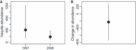
Frequentist inference for vaquita (Phocoena sinus) data. (A) Point estimates and 95% lognormal confidence intervals for vaquita abundance in 1997 and 2008 in the core area of the species’ distribution. (B) Point estimate and 95% normal confidence interval of d = N2008 − N1997, the change in vaquita abundance between 1997 and 2008.
Frequentist inference
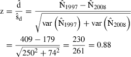
 is the estimated standard error. From the standard normal distribution, P = 0.38 for this z value or larger (two-tailed). Thus, the null hypothesis that 1997 and 2008 abundance was equal is not rejected. In the indirect logic of NHST, P = 0.38 does not mean 1997 and 2008 vaquita abundance was equal, but it does mean that the data were not inconsistent with that assumption. The burden of proof is to show that abundance changed, and the data were not sufficiently improbable to do that. It is frequently emphasized that failing to reject the null hypothesis does not mean that the null hypothesis is true, but when a decision has to be made, this is a distinction without a difference. The practical consequence is that we act as if there was no decline in vaquita abundance.
As an alternative to NHST, many papers suggest approaching the data as an estimation problem rather than as a hypothesis-testing problem (e.g.Jones 1955; Gardner & Altman 1986; Nakagawa & Cuthill 2007). In other words, the primary goal is to estimate effect size and a measure of its uncertainty, such as a confidence interval, not to test the null hypothesis of no change. For the vaquita data, the effect of interest is the change in abundance, d = N2008 − N1997. One estimate of d is the difference of the two point estimates,  , where the negative value indicates that the change was a decrease. The key question is, how certain are we of this estimate? If we assume a normal distribution with standard deviation 261, as computed in the Wald test above, the 95% confidence interval for d extends from −741 to +281 (Fig. 2B). The confidence interval includes 0, which represents the null hypothesis that 1997 and 2008 vaquita abundance was the same.
Confidence intervals and NHST are both frequentist procedures, and they are closely related: if the null hypothesis of no difference is not rejected at the α level, then the 1 − α confidence interval will include 0. Thus, computing a confidence interval does not lead to a different conclusion than NHST about the statistical significance of the results. It does, however, focus attention on the quantity of interest, and thus is more informative than simply reporting a P-value. Looking at Fig. 2B, one is less likely to misstate the NHST result as ‘there was no decline in abundance’. The estimated decline is 230 animals, not 0, although the confidence interval about the estimated decline is large and includes 0. In the case of the thought experiment with two toxins, computing and reporting effect sizes would make it clear that the estimated effect of the second toxin was larger. When there are three or more estimates to be compared simultaneously, a significance test does have the advantage that it gives the overall Type I error rate of falsely rejecting the null hypothesis, a rate not easily shown by confidence intervals.
Confidence intervals, like P-values, are widely misunderstood. Many biologists interpret the 95% confidence interval to mean that we are ‘95% confident’ that the true value is in the interval – for example, the probability is 0.95 that the true change in vaquita abundance is between the upper and lower limits of the vertical line in Fig. 2B. This interpretation of a confidence interval is natural and intuitive but, unfortunately, incorrect. A confidence interval is not that kind of probability interval, which is why Neyman chose a different word for the concept. Rather, calculating a 95% confidence interval is a procedure which, on average, will include the true value ‘95% of the time’. However, the ‘time’ over which this probability applies is the set of all possible realizations of the data, whereas we are interested in the probability that applies to the data we actually have (Goodman 2004b). Like NHST, a confidence interval is a rule for behavior which performs well in a hypothetical long run of data. It does not say anything about the probability of including the true value or of making the correct decision for the data we presently have.
Inference conditional on data
Next we consider methods of reaching conclusions which are conditional on the data, rather than conditional on a hypothesis. Unlike NHST, these methods indicate the degree of support for the hypothesis that vaquitas decreased in abundance. The degree of support can be measured in terms of likelihood ratios (likelihood inference), probability (Bayesian inference) or information theory (model-based inference). For discussion of other alternatives, see Good (1992), Lecoutre et al. (2001) and Berger (2003). We also consider two approaches to the data. In the first approach, analysis proceeds in three steps: (i) estimate 1997 abundance, (ii) estimate 2008 abundance, and (iii) compare the two estimates. Inference about change in abundance (the third step) is based on the results of the first two, as in the Wald test above. However, the estimates and their standard errors are summaries of the original data, and some information is lost. In the second approach, we use the original data to estimate abundance and infer change in abundance in a single integrated analysis. Combining data into a single analysis leads to improved inference (Goodman 2004a).
Inference based on summarized data
We assume that line-transect analyses (Buckland et al. 2001) of the 1997 and 2008 data have already been carried out to estimate vaquita abundance in each year. Inference about change in abundance is based on the resulting estimates  ,
,  ,
,  and
and  , where
  is the standard error of the estimate.
Likelihood inference

The joint likelihood L may be plotted as a function of its two parameters, the change in abundance d and vaquita abundance in 1997 N1997. The likelihood surface has a diagonal ridge, indicating that the likelihoods of d and N1997 are negatively correlated (Fig. 3A). Our focus is to judge support for change in abundance d; N1997 is a so-called nuisance parameter, a parameter of secondary interest which is necessary to estimate in order to make inference on the parameter of primary interest, d. There are various ways to obtain the likelihood of a parameter of interest which is influenced by other parameters (Royall 1997, Chap. 7). A common method is to use, for each value of d, the maximum of the likelihoods computed over all values of N1997 (Fig. 3B). This is called the profile likelihood because it is the profile of the likelihood surface viewed from the d axis. The mean of this function is near −230, as expected, but the maximum is at d = −113.
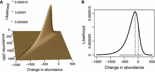
Likelihood inference for d = N2008 − N1997, the change in vaquita abundance between 1997 and 2008, for summarized data. (A) Joint likelihood surface of d and N1997. (B) Profile likelihood of d. The horizontal gray line is the 1/8 likelihood interval. The dotted vertical lines indicate the maximum likelihood at d = −113 and the likelihood at d = 0.
Given the likelihood of d (Fig. 3B), inference can be based on the ratio of the likelihoods of any two values of d. For example, the likelihood ratio against the hypothesis of no change is L(d = −113)/L(d = 0) = 0.0000156/0.0000109 = 1.44 (ratio of heights of vertical dotted lines in Fig. 3B). A likelihood ratio of 1.44 means the data provide more evidence for a change of −113 vaquitas than for a change of 0, but only weakly so.
Inference could also be based on the range of d values for which the data provide evidence of a given strength. Royall (1997, p. 11–12) suggests, for example, that a likelihood ratio of 8 could be interpreted as moderate evidence, intuitively equivalent to the ratio of evidence in favor of a two-headed coin over a fair coin when 3 (23 = 8) consecutive heads have been observed. A likelihood interval of d values for which there is this degree of support extends from −666 to +142 (horizontal gray line in Fig. 3B). Values of d inside this interval have likelihood ratios >1/8 and values outside this interval have likelihood ratios <1/8.
Bayesian inference


We initially assume a uniformly flat surface for the joint prior, which means that we assume all values of N1997 and N2008 are equally probable in each year, and that there is no correlation between them.5 The result is the joint posterior probability distribution of N1997 and N2008 shown in Fig. 4. The marginal posteriors of N1997 and N2008 are obtained by integrating the joint posterior for each variable (Fig. 5A). The distribution of d = N2008 − N1997 can be obtained by sampling the joint posterior distribution.6 As expected with uniform priors in this simple case, the posterior of d (Fig. 5B) is similar to the likelihood of d (Fig. 3B), with a mean of −225 and a maximum value at d = −94. They are not exactly the same shape because Fig. 3B is a profile of the likelihood function, whereas Fig. 5B is proportional to the marginal integral of the likelihood function.

Joint relative posterior probability of N1997 and N2008 for Bayesian analysis of the summarized vaquita data, scaled to the maximum value.
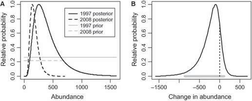
Bayesian inference for summarized vaquita data with noninformative priors. Distributions are scaled to the maximum value of the posteriors. (A) Prior and posterior distributions of N1997 and N2008. Priors are scaled to have the same area as the posterior for the same year. (B) Posterior distribution of change in abundance d = N2008 − N1997. The horizontal gray line is the central 95% probability interval, and the vertical dotted line at d = 0 indicates the fractions of the distribution above and below 0.
Despite the similarity in shape of 3, 5, there is an important conceptual difference: the posterior is a probability distribution, whereas the likelihood is not. This has consequences for inference. A probability distribution is an absolute measure of support, but likelihood ratios (and, later, information-theoretic differences) provide relative measures of support among two or more hypotheses. We can compute an interval which has a probability of 0.95 of including the true value, i.e. what many people incorrectly think a 95% confidence interval is giving them. Posterior probability intervals are also called credibility intervals. A central 95% probability interval for the change in vaquita abundance extends from −864 to +111 (horizontal gray line in Fig. 5B). The central 95% probability interval contains equal probabilities in the upper and lower tails of the distribution, but other intervals may be used. The shortest interval is called the highest posterior density interval. We can also compute Pr(d < 0) = 0.88, that is, the probability of a decrease of any amount (fraction of the area under the curve to the left of the vertical dotted line in Fig. 5B). Another informative statistic is the odds of a decrease Pr(d < 0)/Pr(d > 0) = 0.88/0.12 ≅ 7. In other words, it is seven times more probable that vaquita abundance decreased than that it increased.
A useful but sometimes controversial feature of Bayesian methods is the use of prior information. It is useful because additional information from previous or related studies can be brought seamlessly into the analysis for stronger inference. It can be controversial because conclusions may depend not on current data alone, but on a combination of current data and additional information brought from other studies. Here we will not discuss the issue but simply illustrate the use of informative priors and show that they modify the posteriors.
Prior to the 1997 survey, there was some knowledge of vaquita abundance based on previous partial surveys in the area (Barlow et al. 1997). Likewise, prior to the 2008 survey, there were indications that the population could be as small as 150, based on increased fishing effort and the bycatch rate in gillnets (Jaramillo-Legorreta et al. 2007). For the sake of this example, we do not attempt a detailed analysis, ignore some issues of independence, and simply assume reasonable prior means of 600 and 150 for 1997 and 2008, respectively, with large uncertainty (CV = 100%), based on these previous data. With these informative lognormal priors, the marginal posteriors of N1997 and N2008 (Fig. 6A) are narrower and slightly different in position than the posteriors with uniform priors (Fig. 5A). The posterior of d (Fig. 6B) is also narrower than the previous estimation (Fig. 5B). As a result, the central 95% probability interval is smaller, from −622 to +51 (horizontal gray line in Fig. 6B), the probability of a decrease Pr(d < 0) = 0.93 is larger (fraction of area under the curve to the left of the vertical dotted line in Fig. 6B), and the odds of a decrease 0.93/0.07 ≅ 13 are higher. These differences are due to the additional information brought to the analysis in the priors.
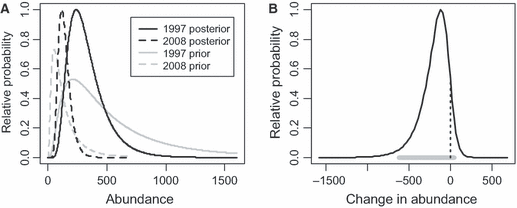
Bayesian inference for summarized vaquita data with informative priors. Distributions are scaled to the maximum value of the posteriors. (A) Prior and posterior distributions of N1997 and N2008. Priors are scaled to have the same area as the posterior for the same year. (B) Posterior distribution of change in abundance d = N2008 − N1997. The horizontal gray line is the central 95% probability interval, and the vertical dotted line at d = 0 indicates the fractions of the distribution above and below 0.
In either case, the results of Bayesian analyses are somewhat different than the conclusions of the previous frequentist and likelihood analyses of the summarized data. The odds that vaquita abundance decreased between 1997 and 2008 are moderately strong – 13 or 7, depending on whether we want to base inference on the additional data in the priors or not.
Inference based on original data
The original line-transect data were the number of km surveyed each year, the number of vaquita sightings each year, and group size and distance from the trackline for each sighting. There are five parameters to estimate instead of two: d, N1997, g, f1997 and f2008, where the latter three are additional nuisance line-transect parameters needed to estimate abundance in each year. Because standard line-transect software (Thomas et al. 2010) uses a combination of likelihood and non-likelihood methods, we use the full likelihood approach of Eguchi & Gerrodette (2009) to compare methods of inference. See Gerrodette et al. (2011) for more details of the application to these data.
Likelihood inference
The five-dimensional joint likelihood equivalent of Fig. 3A would be difficult to plot, but our focus is on d, the change in abundance. The profile likelihood of d based on original data (Fig. 7A) is narrower than the profile likelihood based on summarized data (Fig. 3B). The maximum likelihood estimate is d = −224 vaquitas, and the likelihood ratio against a change of 0 is L(d = −224)/L(d = 0) = 2.5 × 10⁸. This is extremely strong evidence that vaquita abundance decreased, intuitively equivalent to the strength of evidence in favor of a two-headed coin over a fair coin when log2(2.5 × 10⁸) = 24.6 consecutive heads have been observed. The 1/8 likelihood interval extends from −840 to −168 (horizontal gray line in Fig. 7A).
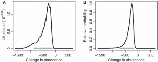
Likelihood and Bayesian inference on d = N2008 − N1997, the change in vaquita abundance between 1997 and 2008, using original data. (A) Profile likelihood of d. The horizontal gray line is the 1/8 likelihood interval. (B) Posterior distribution of d, scaled to the maximum value. The horizontal gray line is the central 95% probability interval.
Bayesian inference
For the integrated Bayesian analysis, uniform priors were used for all parameters except g (Gerrodette et al. 2011). The posterior of d (Fig. 7B) is much narrower than the posterior based on summarized data with uniform priors (Fig. 5B), and all of the probability density is less than zero. The maximum probability occurs at a change of d = −220 vaquitas, the median value at d = −313, and the central 95% probability interval extends from −707 to −175. The probability of a decrease is Pr(d < 0) > 0.9999999, and the odds of a decrease are Pr(d < 0) / Pr(d > 0) = 1.8 × 10⁹.
Model-based inference


 of the parameters. The AIC difference between the models is ΔAIC = 32.1. An AIC difference of 3 already indicates much less support, so a difference of 32.1 indicates very little support for the no-change-in-abundance model. Support can also be judged in terms of model weights. The Akaike weights of the two models are


Conclusion
Different methods of statistical inference use different metrics and can give quantitatively and qualitatively different results (Table 1). Support for a hypothesis can be measured in terms of information theory, likelihood ratios or probability. The concept of likelihood conditional on data is central to inference, although model-based, likelihood and Bayesian inference use likelihood in different ways. Modern statistical methods allow multiple types of data to be combined into a single analysis for improved inference. In the case of the vaquita data, there was a substantial loss of information when summarized data (estimates and standard errors) were used to infer change in abundance. Integrated analyses based on the original data had less uncertainty (Fig. 7) and indicated much stronger support for the conclusion that there was a decrease in abundance (Table 1). All of the alternatives to NHST were more informative about ‘what the data say’ than the P-value and its associated significance.
Fifty years ago, Rozeboom (1960) wrote that his criticism of NHST was ‘not a particularly original view’, and that ‘the traditional null-hypothesis procedure has already been superceded [sic] in modern statistical theory by a variety of more satisfactory inferential techniques’. Fifty years on, would that this were so.
Footnotes
Acknowledgements
Paul Dayton never claimed expertise in statistics, but he always encouraged challenges to accepted thinking. The paper was improved by the contributions of Frederick Archer, Tomoharu Eguchi, Daniel Goodman, Jeffrey Laake, Iliana Ruiz-Cooley and George Watters, although this does not necessarily mean that they agree with all the views expressed. Alan Jackson assisted with the preparation of the web page listing papers discussing NHST since 2001. Constructive comments by Lee Eberhardt and two anonymous reviewers clarified and improved the presentation.


